5Methods: Generating predicted maize grain Se concentration for Malawi
Here, we describe all the steps performed to obtain the prediction of maize grain Se concentration in unsampled location of Malawi. The R script (01_maize-model.R) used to run the analysis can be found in the accompanying repository and are an adaptation of the script developed by Prof Murray Lark for the GeoNutrion project which are published here.
CEPHaStat version  3

CEPHaStat is a collection of R functions produced by the UKRI GCRF
CEPHaS project.  The functions relate primarily to statistical analysis of
soil and related data from agricultural and environmental surveys and
experiments.  The CEPHaStat file can be shared as it stands, and is made
available to all for use, without warranty or liability.
Code
# Note that the script contains an adaptation of the scripts develop for # the analysis of the Malawi and the Ethiopia data sets (GeoNutrition)# Loading the datadata.df <-readRDS(here::here("data", "inter-output", "mwi-grain-se_raw.RDS")) # cleaned geo-loc maize Se data (2 datasets)
5.1 Exploratory analysis
The data set that we are using is the output generated in the script (00_cleaning-maize.R) which contains the information on crop Se concentration in Malawi. The variables are the GPS sample location (lat/lon), maize grain Se concentration, soil pH and Mean Annual Temperature (MAT) of the two combined datasets (Kumssa et al. (2022), Chilimba et al. (2011)) See Chapter 4 for more information on the data set.
Then, information for maize only is selected, and some housekeeping actions are performed, such as, removing missing values for the variable of interest (Se_raw) which contains the Se concentration including below detection limits, and transforming zeros into the minimum value. This last operation is performed as log-transformation would be required in subsequent steps.
Code
## Choosing only entries with maize Se valuesdata.df <-subset(data.df, Crop =="Maize")# Housekeeping: Check NA and zerossum(is.na(data.df$Se_raw))
[1] 7
Code
sum(data.df$Se_raw ==0&!is.na(data.df$Se_raw))
[1] 23
Code
data.df <-subset(data.df, !is.na(Se_raw) & Se_raw>0) #excluding NA & zeros
Note
Zeros were excluded due to:
Assumed that maize sample did not contain Se
Log-transformation of zero is equal to -Inf.
Now, we are performing some summary statistics and checking the data skewness to decide on the log-tranformation.
Code
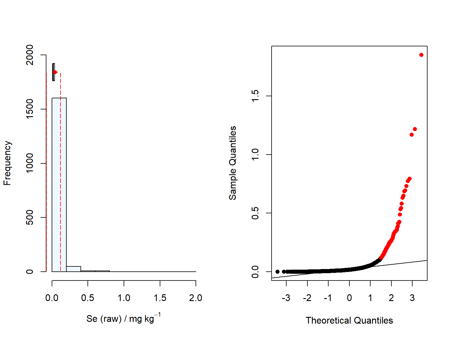
# Now create plot name with Se (element of interest)element<-"Se_raw"Crop.target <-"maize"plotname<-expression("Se (raw) /"~mg~kg^{-1})plotname2<-expression("Se (raw) /"~log~mg~kg^{-1})# Compute summary statistics of the selected variabledata.df <-as.data.frame(data.df)summary<-(summa(data.df[,element]))summary<-rbind(summary,(summa(log(data.df[,element]))))row.names(summary)<-c("mg/kg,","log mg/kg")summaplot((data.df[,element]),plotname)
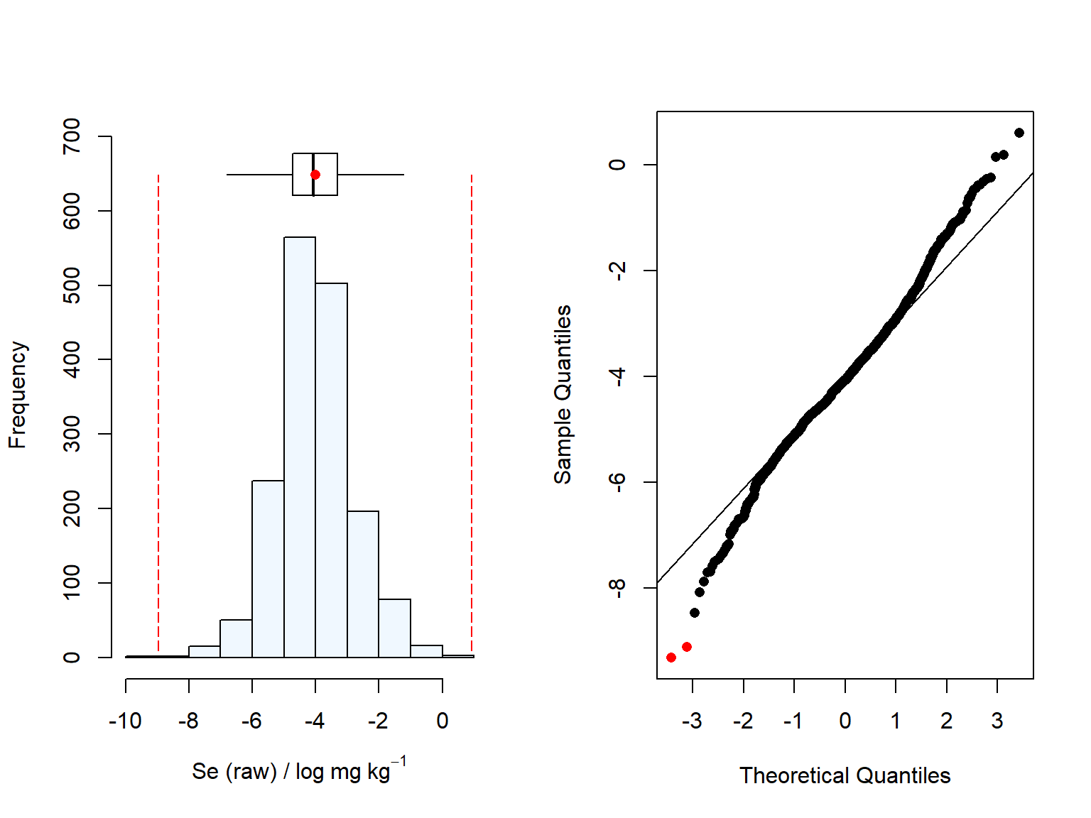
Due to the markedly right-side skewness, we decided to log-transform the variable (Se_raw). We can see in the figure below, that the log-transformed concentration of Se in maize is very close to normality, hence we will proceed with the log-trasformed variable for the variogram estimation. Variograms are particularly sensitive to right-side outliers (e.g., exceptionally large values) (Webster and Oliver (2007)).
Code
# Checking the data distribution after log-transformationsummaplot(log(data.df[,element]),plotname2)
Code
# Log-transforming the maize Se conc.data.df[,element]<-log(data.df[, element]) plotname<-plotname2
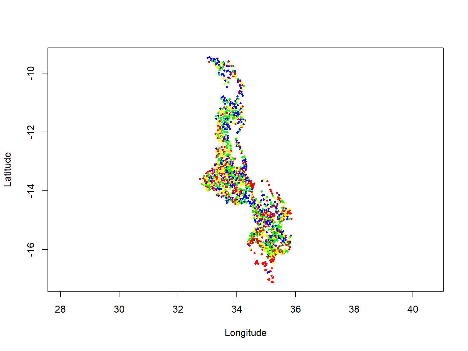
Then, we can see in Figure 5.1 the log-transformed maize Se concentration coloured by their quartile from the smallest (in blue) to the highest (in red) to see if there are some spatial trend or pattern. We also checked for North to South and West to East trends (see code in the R scripts).
Code
# Map of maize Se concentrationquantiles<-as.character(cut(data.df[,element],quantile(data.df[,element],c(0,0.25,0.5,0.75,1)),include.lowest=T,label=c("blue","green","yellow","red"))) # Classified post-plotoptions(scipen=5)plot(data.df[,"Longitude"],data.df[,"Latitude"], # Lon & Lat variablespch=16,col=quantiles,asp=1,xlab="Longitude",ylab="Latitude",cex=0.5)
Figure 5.1: Map of Malawi: each point represents the maize Se concentration (log-transformed) at a sampled location, the colours show the quantiles: 0-24.9% (blue), 25-49.9% (green), 50-79.9% (yellow), 75-100% (red)
5.2 Variogram estimation and validation
After the data exploration, the next step is selecting the best estimators to fit the model (ordinary kriging (OK)) for getting the most accurate results.
The method for evaluating and selecting the model was based on Gashu et al. (2021) and best practices suggested by and Webster and Oliver (2007).
5.2.1 Obtaining the variogram estimates
In this section, we are studying the spatial structure of the data by generating an empirical variogram.
To do so, first we need to calculate some information from the data: the distance between all pairs of observations (lag) and the difference in maize Se concentration between two observations (varogram cloud).
Code
# Exploratory study of empirical variogram# Make a variogram cloudN<-nrow(data.df) # No. of observationsNP<-0.5*N*(N-1) # No. of pairs# Extracting variables from the data setLong<-data.df$Longitude # LonLat<-data.df$Latitude # Latz<-data.df[,element] # maize Se conc.# Generating vectors to store the data to be calculated in the loop belowlag<-vector("numeric",NP) # Distance between 2pts (lag)vclo<-vector("numeric",NP) # Variogram cloud bear<-vector("numeric",NP) # Shortest distance between 2pts (on an ellipsoid or sphere)ico=0for (i in1:(N-1)){for (j in (i+1):N){ico=ico+1# print(ico/NP)lag[ico]<-distVincentySphere(c(Long[i],Lat[i]),c(Long[j],Lat[j]))/1000#bear[ico]<-finalBearing(c(Long[i],Lat[i]),c(Long[j],Lat[j]), a=6378137, f=1/298.257223563, sphere=TRUE)zi<-(z[i])zj<-(z[j])vclo[ico]<-(zi-zj)}}
With that information, we are going to decide on the maximum lag distance that will be included in the variogram, and the lag bins. For more information about the use of bin distance (d) and the importance of its selection, see “Irregular sampling in one dimension” (Webster and Oliver (2007), page 68).
Code
# Setting for the variogram:# max. distance (e.g., end of spatial correlation) around 100km # We have tested 100km, 150km and 200km maxdist <-100lagbins<-cut(lag,seq(0,maxdist,10),labels=seq(5,maxdist,10)) # 10-km bins for Malawilag2<-lag[!is.na(lagbins)]vclo2<-vclo[!is.na(lagbins)]lagbins<-factor(lagbins[!is.na(lagbins)])nlags<-nlevels(lagbins)
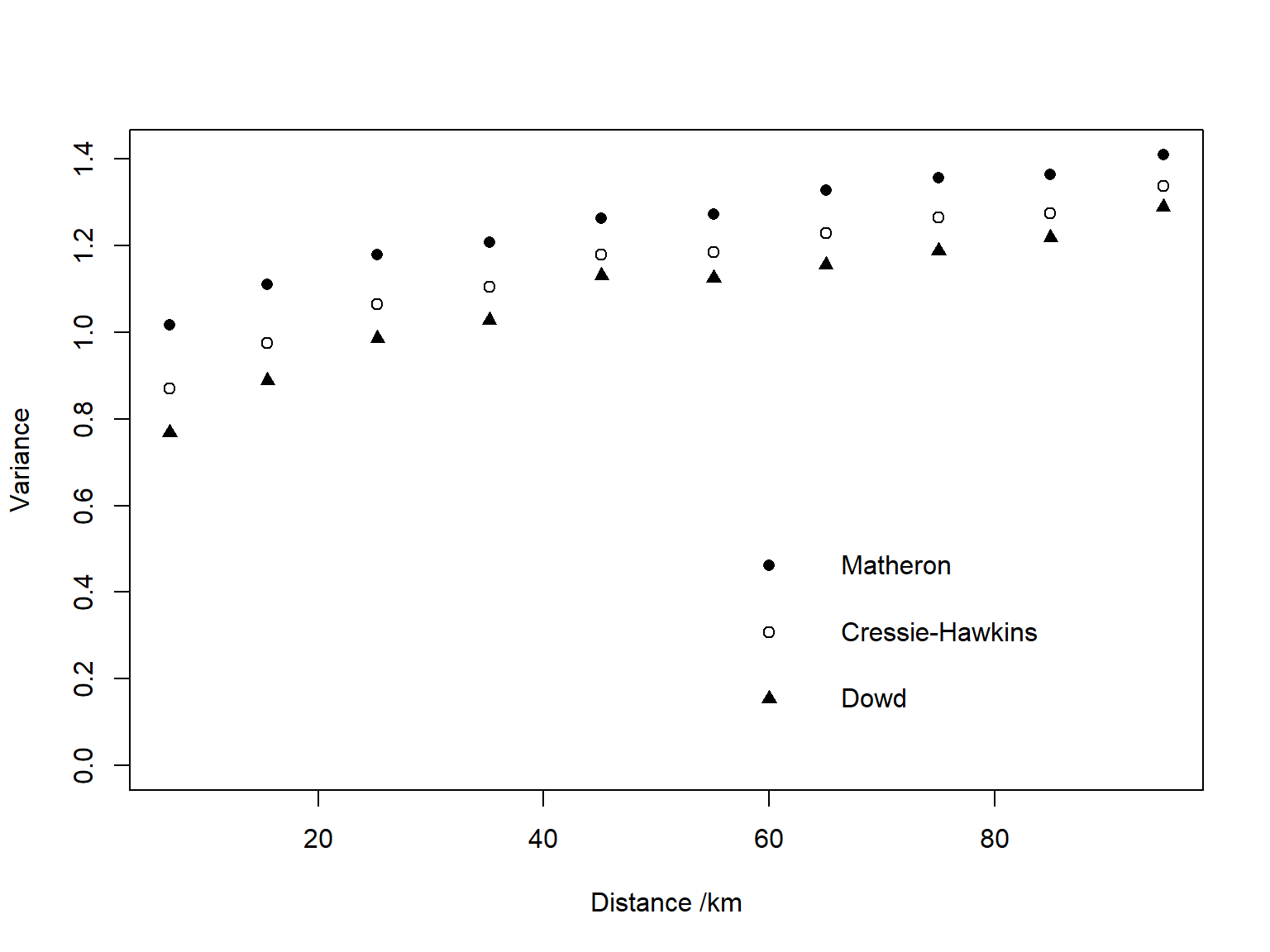
Then, calculating the semi-variance we are using three different estimators: isotropic Matheron (Ma), Cressie-Hawkins (CH) and Dowd (Do).
In order to store the data we created three matrices, one semivar which contains the variogram estimates and was structured as follow:
column 1 are estimates with Matheron (iso-Ma),
columns 2 are for the robust estimator Cressie-Hawkins (iso-CH),
columns 3 are for the robust Dowd estimator (iso-Do).
Then, the lag pairs per bin, and the mean lag distance were stored in the objects npair and varlag (isotropic).
Code
# Matrices for storing the resultssemiv<-matrix(nrow=nlags,ncol=3)npair<-matrix(nrow=nlags,ncol=1)varlags<-matrix(nrow=nlags,ncol=1)colnames(semiv)<-c("iso-Ma","iso-CH","iso-Do")colnames(npair)<-c("iso")colnames(varlags)<-c("iso")
Now the mean distance per lag bin and the number of pairs in each lag (total/mean = n) and the estimators are calculated.
Code
# Adding the mean lag distance per bin varlags[,1]<-as.numeric(by(lag2, lagbins, mean))# Adding the number of pairs in each lag bin npair[,1]<-as.numeric(by(lag2, lagbins, sum))/as.numeric(by(lag2, lagbins, mean))# Calculating the estimator# Matheronsemiv[,1]<-0.5*(as.numeric(by((vclo2)^2, lagbins, mean)))# CHsemiv[,2]<-(as.numeric(by((sqrt(abs(vclo2))), lagbins, mean)))^4semiv[,2]<-0.5*semiv[,2]/(0.457+0.459/npair[,1]+0.045/npair[,1]^2)# Dovclo2d<-c(vclo2,-vclo2)lagbinsd<-c(lagbins,lagbins)semiv[,3]<-0.5*(as.numeric(by(vclo2d, lagbinsd, mad)))^2
And then, results are plotted…
Code
# Now plot the variogramsmaxv<-max(semiv[,1:3])minv<-min(semiv[,1:3])plot(varlags,semiv[,1],ylim=c(0,maxv),xlab="Distance /km",ylab="Variance",pch=16)points(varlags,semiv[,2],pch=1)points(varlags,semiv[,3],pch=17)locsv<-minv*c(0.6,0.4,0.2)points(60,locsv[1],pch=16)points(60,locsv[2],pch=1)points(60,locsv[3],pch=17)text(65,locsv[1],"Matheron",pos=4)text(65,locsv[2],"Cressie-Hawkins",pos=4)text(65,locsv[3],"Dowd",pos=4)
5.2.2 Fit exponential variogram functions to each set of estimates
First, we need to choose initial estimates for the parameters. These will impact the estimates, so also should they be chosen with care! (See Chapter 6 and page 101 of Webster and Oliver (2007)).
Code
# Reasonable initial estimates of the parameters must be entered belowco<-20000c1<-30000a<-50maxl<-max(varlags)*1.1par(mfrow=c(2,2))
Then, we are fitting the model using the different estimators using weighted least squares (See the wls() function in the kringing-functions.R script under the functions folder).
Code
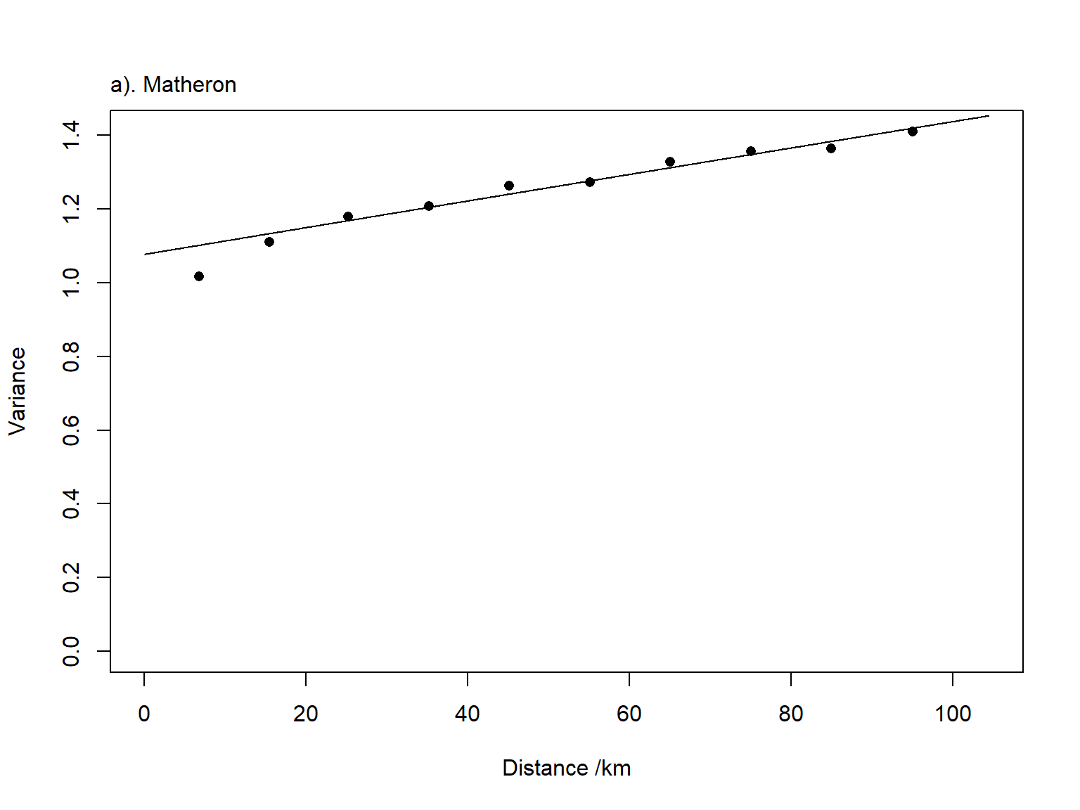
# Matheron's estimator (Ma)h<-varlags[,1] # mean lag distance per bin sv<-semiv[,1] # Ma semivariancenpa<-npair[,1] # No of pairs per binkap<-0.5# Fitting the model oo<-optim(c(co,c1,a),wls,method="L-BFGS-B",lower=c(0.0,0.0,0),upper=c(1000000,1000000,5000))Ahat<-length(h)*log(oo$value)+6ooMa<-oo # Storing values
Visually inspecting the results of the fitted variogram for the Matheron’s estimator.
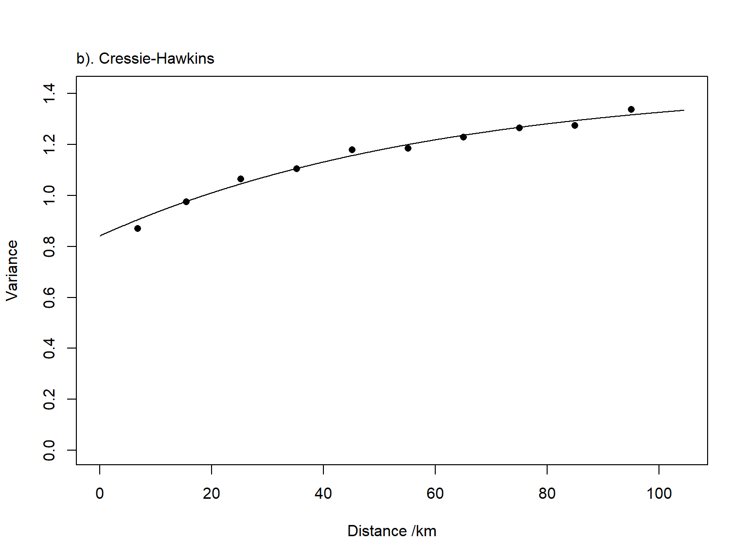
Then, we fitted the varigram using the Cressie’s and Hawkins’s estimators.
Code
# Cressie's and Hawkins's estimator (CH)h<-varlags[,1] # mean lag distance per bin sv<-semiv[,2] # CH semivariancenpa<-npair[,1] # No of pairs per binkap<-0.5# Fitting the model oo<-optim(c(co,c1,a),wls,method="L-BFGS-B",lower=c(0.0,0.0,0),upper=c(1000000,1000000,5000))Ahat<-length(h)*log(oo$value)+6ooCH<-oo # Storing values
Again, we proceed to visually inspect the fitted variogram.
Code
# Plotting the dataplot(varlags[,1],semiv[,2],ylim=c(0,maxv),xlim=c(0,maxl),xlab="Distance /km",ylab="Variance",pch=16)lines(seq(0,maxl,0.1),oo$par[1]+oo$par[2]*(1-exp(-seq(0,maxl,0.1)/oo$par[3])))mtext("b). Cressie-Hawkins",3,adj=0,line=0.5)
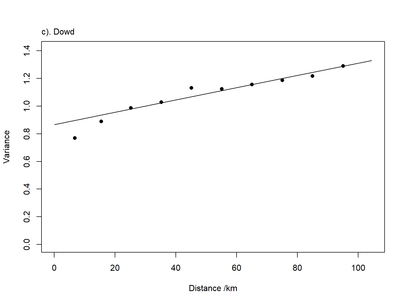
And, finally, we fitted the variogram using the Dowd’s estimator.
Code
# Dowd's estimator Doh<-varlags[,1] # mean lag distance per bin sv<-semiv[,3] # Do semivariancenpa<-npair[,1] # No of pairs per binkap<-0.5# Fitting the model oo<-optim(c(co,c1,a),wls,method="L-BFGS-B",lower=c(0.0,0.0,0),upper=c(1000000,1000000,5000))Ahat<-length(h)*log(oo$value)+6ooDo<-oo # Storing values
Cross-validation consists in estimating the sample points at a time by leaving one observation out. It was performed using a subset of the data, for our case, we used 1,000 observations.
Code
N<-nrow(data.df) # No. of observationsNv<-500# vs 1000 check perc.kvop<-matrix(nrow=Nv,ncol=5)Nr<-Nv-1# Make random sample without replacementsam<-sample(1:N,Nv,replace=F)# Sub sample dataLong_s<-Long[sam]Lat_s<-Lat[sam]z_s<-(z[sam])
After, getting the subset of the sample, we repeat the step 1 just for the sub-sample, i.e, calculating the distance matrix (e.g., pair distances).
Code
# Compute distance matrix for subsampleDM<-matrix(0,nrow=Nv,ncol=Nv)for (i in1:(Nv-1)){for (j in (i+1):Nv){DM[i,j]<-distVincentySphere(c(Long_s[i],Lat_s[i]),c(Long_s[j],Lat_s[j]))/1000#WGS84 ellipsoid is used by defaultDM[j,i]<-DM[i,j]}}
Now, we are performing the cross-validation for the three estimators.
First, we chose the parameters of the model fitted using the Matheron estimator.
Code
#Select parameter set to validateooX<-ooMa # Matheron# variogram matrixGam<-ooX$par[1]+ooX$par[2]*(1-matern(DM,ooX$par[3],0.5))diag(Gam)<-0for (i in1:Nv){# print(i)A<-Gam[-i,-i]A<-cbind(A,rep(1,Nr))A<-rbind(A,c(rep(1,Nr),0))z_0<-z_s[i]z_n<-z_s[-i]b<-c(Gam[i,-i],1)lam<-solve(A)%*%bZhat<-sum(z_n*lam[1:Nr])err<-z_0-Zhatkv<-t(b)%*%lamtheta<-(err^2)/kvkvop[i,]<-c(z_0,Zhat,err,kv,theta)}
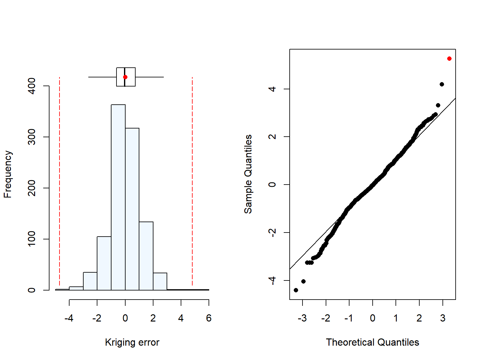
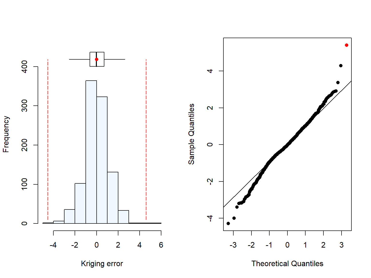
Then, an exploratory plot of prediction errors is produced for the variogram, and store the validation outputs for later use.
Code
# Visualising the error dev.new()summaplot(kvop[,3],"Kriging error")# Storing the valueskvopMa<-kvopcolnames(kvopMa)<-c("z_0","Zhat","err","kv","theta")
Then, we repeated the same operation for the model fitted with Cressie & Hawkins estimator.
Code
#Select parameter set to validateooX<-ooCH# variogram matrixGam<-ooX$par[1]+ooX$par[2]*(1-matern(DM,ooX$par[3],0.5))diag(Gam)<-0for (i in1:Nv){# print(i)A<-Gam[-i,-i]A<-cbind(A,rep(1,Nr))A<-rbind(A,c(rep(1,Nr),0))z_0<-z_s[i]z_n<-z_s[-i]b<-c(Gam[i,-i],1)lam<-solve(A)%*%bZhat<-sum(z_n*lam[1:Nr])err<-z_0-Zhatkv<-t(b)%*%lamtheta<-(err^2)/kvkvop[i,]<-c(z_0,Zhat,err,kv,theta)}
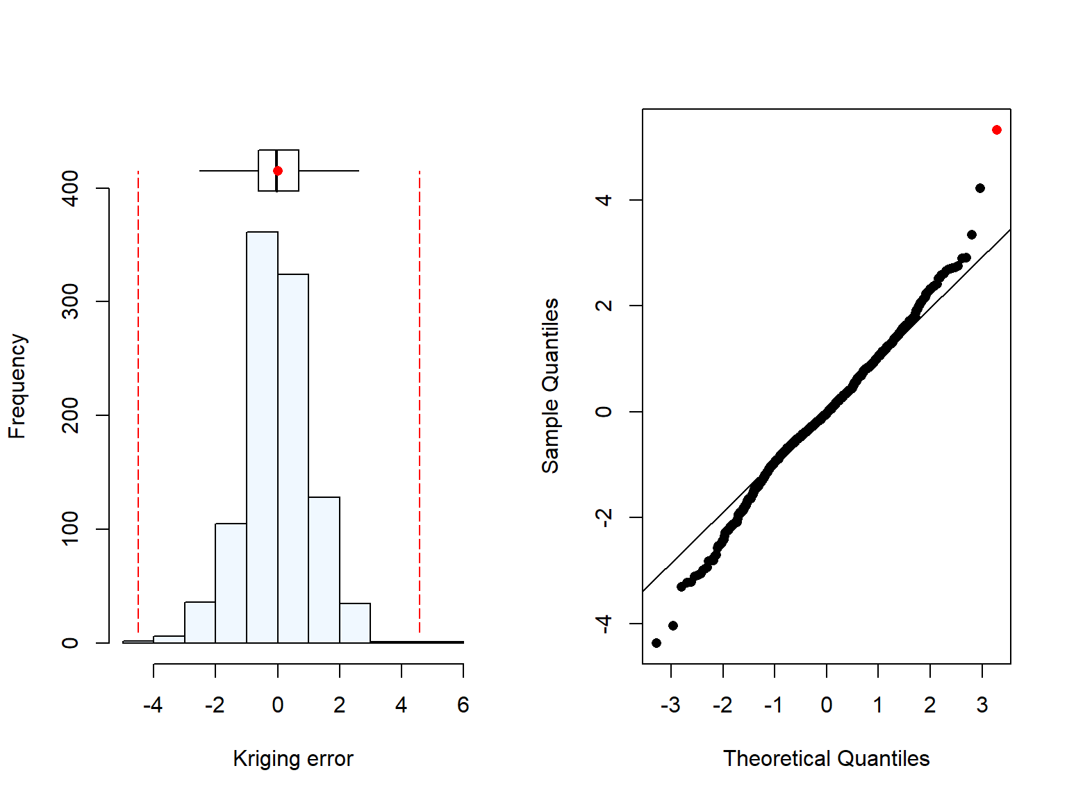
And, visusalise and store the values.
Code
# Visualising the errordev.new()summaplot(kvop[,3],"Kriging error")# Storing the valueskvopCH<-kvopcolnames(kvopCH)<-c("z_0","Zhat","err","kv","theta")
Finally, we repeated the operation for Dowd.
Code
#Select parameter set to validateooX<-ooDo# variogram matrixGam<-ooX$par[1]+ooX$par[2]*(1-matern(DM,ooX$par[3],0.5))diag(Gam)<-0for (i in1:Nv){#print(i)A<-Gam[-i,-i]A<-cbind(A,rep(1,Nr))A<-rbind(A,c(rep(1,Nr),0))z_0<-z_s[i]z_n<-z_s[-i]b<-c(Gam[i,-i],1)lam<-solve(A)%*%bZhat<-sum(z_n*lam[1:Nr])err<-z_0-Zhatkv<-t(b)%*%lamtheta<-(err^2)/kvkvop[i,]<-c(z_0,Zhat,err,kv,theta)}
And, visualising and storing.
Code
# Visualising the errordev.new()summaplot(kvop[,3],"Kriging error")#summa(kvop[,5])# Storing the valueskvopDo<-kvopcolnames(kvopDo)<-c("z_0","Zhat","err","kv","theta")
We then checked the mean and median standardised squared prediction error for each variogram.
The median for Matheron was just outside the median standardised squared prediction error interval (thetaCLL, thetaCLU) calculated below. Then, when we compared the other robust estimators, both medians were in range, with Dowd closest to 0.455.
Code
# checking the theta (MSER)summa(kvopMa[,5])[,c(1,2)]summa(kvopCH[,5])[,c(1,2)]summa(kvopDo[,5])[,c(1,2)]thetaCLU<-0.455+2*sqrt(1/(8*(Nv/2)*(dchisq(0.455,1))^2))thetaCLL<-0.455-2*sqrt(1/(8*(Nv/2)*(dchisq(0.455,1))^2))print(c(thetaCLL,thetaCLU))
Hence that was the model parameters chosen for the kriging predictions at unsampled locations.
Code
# For our maize Se data (log-transformed) Do was# the better performingooX<-ooDo
Validation outputs were saved for the estimators of Matheron (kvopMA), Cressie & Hawkins (kvopCH) and Dowd (kvopDo) respectively (see R script:01_maize-model.R).
5.3 Predicting maize grain Se concentrations in unsampled locations
After choosing the optimal estimator, we used it for predicting the maize Se concentration in unsampled locations in Malawi using ordinary kriging.
First, we need to load the target locations, which are all the unsampled locations in Malawi (n=178,040). It was obtained by dividing the country in even squares at resolution.
Then, we need to calculate the matrix distance (i.e., the distance between each point location in our target sample) and the variogram matrix for the sampled data as performed previously.
Code
# Loading the data with the unsampled locationstargets.df<-read.csv(here::here("data", "maize", "Malawi_targets.csv"),header=T) # Sampled location dataurdata.df<-data.frame(cbind(Lat,Long,z))# Make a distance matrix among all data points Long<-urdata.df$LongLat<-urdata.df$LatDM<-matrix(0,nrow=N,ncol=N)for (i in1:(N-1)){for (j in (i+1):N){DM[i,j]<-distVincentySphere(c(Long[i],Lat[i]),c(Long[j],Lat[j]))/1000#WGS84 ellipsoid is used by defaultDM[j,i]<-DM[i,j]}}# variogram matrixGam<-ooX$par[1]+ooX$par[2]*(1-matern(DM,ooX$par[3],0.5))A<-GamA<-cbind(A,rep(1,N))A<-rbind(A,c(rep(1,N),0))Ainv<-solve(A)
We prepared the unsampled data set for making the prediction.
Code
# No of unsampled obs.Nt<-nrow(targets.df)# Matrix to store the data from the OKkrop<-matrix(nrow=Nt,ncol=5)# Binding all the sampled locationsAllpoints<-cbind(Lat,Long)
Finally, we performed the prediction. Note that the outputs are the locations (Long/Lat), the log-tranformed predicted value for each location, the log-transformed kriging variance and the Lagrange multiplier. The later one is important because as reported previously (Webster and Oliver (2007)), the back transformation of the lognormal kriging for ordinary kriging need to be done using the following Equation 5.1:
Where \(Z_{OK}(x_0)\) is the back transformed variable at a given point location \((x_0)\), \(Y_{OK}(x_0)\) and \(Var_{OK}(x_0)\) are the kriged estimated log-transformed of the maize Se concentration and its variance using ordinary kriging at the same location, respectively, and \(\lambda(x_0)\) is the Lagrange multiplier.
Note that the prediction will take some time to run, hence, after finishing, we will save the file, before proceeding to back-transforming the data.
Code
# OK predictionfor (it in1:Nt){print(c(it,Nt))# Extract Lat and Long of target point Lat_t<-targets.df$Lat[it]Long_t<-targets.df$Long[it]Bd<-matrix(nrow=(N+1),ncol=1)for (j in1:N){Bd[j]<-distVincentySphere(c(Long[j],Lat[j]),c(Long_t,Lat_t))/1000}#maxdis<-max(Bd[1:Ne])#print(c(it,it/Nt,maxdis))Bd[1:N]<-ooX$par[1]+ooX$par[2]*(1-matern(Bd[1:N],ooX$par[3],0.5))Bd[N+1]<-1lam<-Ainv%*%BdZhat<-sum(z*lam[1:N])kv<-t(Bd)%*%lamlagr<-lam[N+1]krop[it,]<-c(Long_t,Lat_t,Zhat,kv,lagr)}# Back-transforming lognormal OKkrop$Zhat_exp <-exp(krop$Zhat + krop$kv/2- krop$lagr)# Saving exponential OKfname<-paste("data/OK/",paste(Sys.Date(), element,"_OK_exp",Crop.target,".csv",sep=""))write.csv(krop,fname,row.names=F)
Finally, we had to back-transform the data and saved the output in the data folder.
Chilimba, Allan D. C., Scott D. Young, Colin R. Black, Katie B. Rogerson, E. Louise Ander, Michael J. Watts, Joachim Lammel, and Martin R. Broadley. 2011. “Maize Grain and Soil Surveys Reveal Suboptimal Dietary Selenium Intake Is Widespread in Malawi.”Scientific Reports 1 (1, 1): 72. https://doi.org/10.1038/srep00072.
Gashu, D., P. C. Nalivata, T. Amede, E. L. Ander, E. H. Bailey, L. Botoman, C. Chagumaira, et al. 2021. “The Nutritional Quality of Cereals Varies Geospatially in Ethiopia and Malawi.”Nature 594 (7861): 71–76. https://doi.org/10.1038/s41586-021-03559-3.
Kumssa, D. B., A. W. Mossa, T. Amede, E. L. Ander, E. H. Bailey, L. Botoman, C. Chagumaira, et al. 2022. “Cereal Grain Mineral Micronutrient and Soil Chemistry Data from GeoNutrition Surveys in Ethiopia and Malawi.”Scientific Data 9 (1, 1): 443. https://doi.org/10.1038/s41597-022-01500-5.
Webster, Richard, and Margaret A Oliver. 2007. Geostatistics for Environmental Scientists.