7 Model preparation: Maize aggregation and data combination

For the final modelling we are only using predicted maize Se concentration to calculate the different level of aggregation. For more information on the reasons, see the section Model testing & calibration.

The file predmaize.df contains the coordinates of Malawi (lat/lon), the predicted maize Se concentration, both log-transformed (Zhat) and back transformed (Zhat_exp), and their covariance (uncertainty associated to each prediction) for each of the locations in Malawi.

The dataset was derived from the maize.df dataset using ordinary kriging and the scripts can be found in 01_maize-model.R and are based on the study of Gashu and colleagues (2022).

Then, in order to calculate the mean/median value for each level of aggregation we will use the boundaries that were generated in the script (00_cleaning-location.R) and described in Section 3.1.

Code

# Loading libraries and functions -----

#library(plyr) # weighted data analysis
library(dplyr) # data wrangling 
library(stringr) # string data manipulation 
library(ggplot2) # visualisation
library(sf) # spatial data manipulation
library(tmap)  #spatial data manipulation and visualisation


# Data: Shapefiles ----

## Admin Boundaries for Malawi ----

# Reading the EA shapefile w/ updated districts (See 00_cleaning-boundaries.R)
ea_admin <- st_read(here::here( "data", "inter-output", 
                                "boundaries", "mwi_admbnda_adm4_nso.shp"))

Reading layer `mwi_admbnda_adm4_nso' from data source 
  `C:\Users\LuciaSegoviaDeLaRevi\OneDrive - London School of Hygiene and Tropical Medicine\PhD\PhD_r-project\PhD_geospatial-modelling\data\inter-output\boundaries\mwi_admbnda_adm4_nso.shp' 
  using driver `ESRI Shapefile'
Simple feature collection with 10502 features and 14 fields
Geometry type: MULTIPOLYGON
Dimension:     XY
Bounding box:  xmin: 32.67162 ymin: -17.12628 xmax: 35.91842 ymax: -9.363662
Geodetic CRS:  WGS 84

Code

# Changing variable region class to factor
ea_admin$region <- as.factor(ea_admin$region)
                    
# Districts
dist_bnd  <- st_read(here::here( "data",
                                "mwi-boundaries",
                                "mwi_adm_nso_hotosm_20230329_shp", 
                                "mwi_admbnda_adm2_nso_hotosm_20230329.shp"))

Reading layer `mwi_admbnda_adm2_nso_hotosm_20230329' from data source 
  `C:\Users\LuciaSegoviaDeLaRevi\OneDrive - London School of Hygiene and Tropical Medicine\PhD\PhD_r-project\PhD_geospatial-modelling\data\mwi-boundaries\mwi_adm_nso_hotosm_20230329_shp\mwi_admbnda_adm2_nso_hotosm_20230329.shp' 
  using driver `ESRI Shapefile'
Simple feature collection with 32 features and 6 fields
Geometry type: MULTIPOLYGON
Dimension:     XY
Bounding box:  xmin: 32.67164 ymin: -17.12975 xmax: 35.91848 ymax: -9.367346
Geodetic CRS:  WGS 84

Code

dist_bnd <- st_make_valid(dist_bnd) # Check this


# Cluster's EA info
cluster.df <- readRDS(here::here("data", "inter-output", 
                                "dhs_se_gps_admin.RDS"))  %>% 
  distinct(survey_cluster1, EACODE, ADM2_PCODE, ADM2_EN, urbanity)

# Unique EAs where WRA potentially reside
EAselected <- unique(cluster.df$EACODE)

# Loading predicted maize Se conc.

predmaize.df <- read.csv(here::here("data", "OK",
              "2024-05-03Se_raw_OK_expmaize.csv")) %>% 
  rename(predSe = "Zhat_exp")

# Buffer distances
buff.dist <- na.omit(unique(stringr::str_extract(list.files(here::here("data", 
              "inter-output", "boundaries", "buffer")),
                                        "[:digit:]{2}")))

7.1 Data aggregation

Here we are proceeding as described in Section 6.2. In summary, to generate the final aggregations we are:

Loading the boundaries for the administrative units (cluster-level and district-level) and the buffers which can be adapted using the function buffer_generator(), and are 10 km, 15 km, 20 km, 25 km, 30 km, 40 km, 50 km, 60 km. More information on that function can be found in Section 6.2.1.
After selecting the aggregations, we need to get the information on the maize Se concentration for each aggregation area. To do so, we need to convert the predicted maize Se dataset (Long/Lat) into a spatial object (point locations).

Code

# Converting into spatial object
geopredmaize.df <-  st_as_sf( predmaize.df , coords =c("Longitude", "Latitude"),
                              crs = "EPSG:4326")

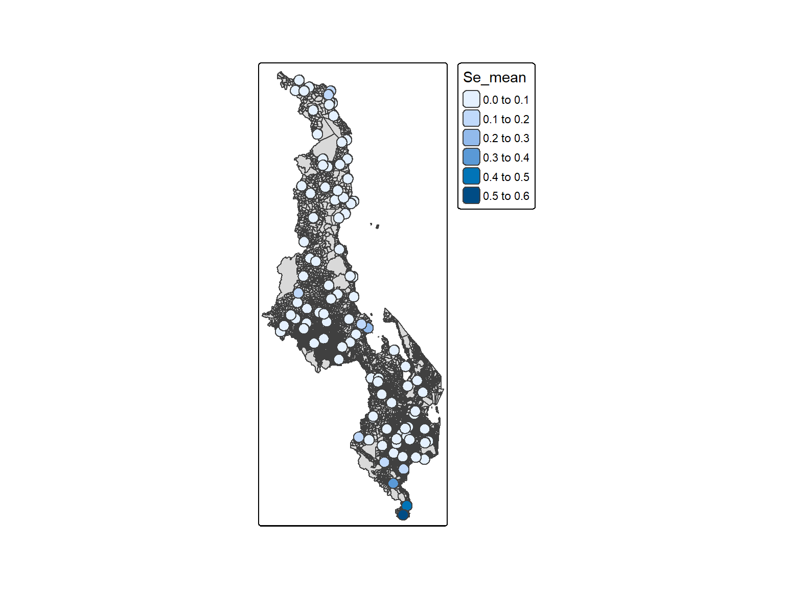
Merging the data by location. This spatial joint allowed us to obtain the maize Se concentration point data in each area. See ?fig-XX.

Note

Because the dataset of the predicted maize is very large, and we only need the maize aggregation for the areas (e.g., EA group) were data on plasma Se were collected, we are using a shapefile with the cluster-level spatial data only for those EAs/clusters with plasma Se concentration collected.

Code

### Cluster ----

## Checking the EAs of the HHs with predicted maize

bnd_reduced <- ea_admin %>% filter(EACODE %in% EAselected)

geopred_ea <-  st_join(geopredmaize.df, bnd_reduced)

Once we know for each maize Se concentration to which EA below, we can aggregate at cluster level (and district) (predmaize).

Code

# Calculating the maize grain Se conc per cluster
predmaize_cluster <- geopred_ea %>% 
  st_drop_geometry() %>% filter(!is.na(ADM2_EN)) %>% 
  right_join(., cluster.df) %>%  filter(!is.na(predSe)) %>% 
  group_by(survey_cluster1) %>% 
  summarise(Se_mean = mean(predSe, na.rm = TRUE), 
            Se_sd = sd(predSe, na.rm = TRUE), 
            Se_median = median(predSe, na.rm = TRUE), 
            Se_iqr = IQR(predSe, na.rm = TRUE), 
            Se_n = n())

For the buffers, it is performed equally but using a loop, that ingest the buffer generated and output the dataset with the maize Se mean for each buffer.

Code

# Getting the distances of the buffers

(buff.dist <- na.omit(unique(stringr::str_extract(list.files(here::here("data", 
              "inter-output", "boundaries", "buffer")),
                                        "[:digit:]{2}"))))

#Saving unti a new object
geodata.df <- geopredmaize.df

# Getting the variable to perform the mean (calculations over)
Se <- grep("Se", names(geodata.df), value = TRUE)

# Looping over the buffers
for(i in 1:length(buff.dist)){
  
  buffer  <- st_read(here::here("data", "inter-output",
                                "boundaries", "buffer",
                                paste0("mwi_buffer", buff.dist[i], ".shp"))) %>% 
    rename(survey_cluster1 = "srvy_c1")
  
  maize_buff <- st_join(geodata.df, buffer) 
  
if(sum(is.na(maize_buff[,Se]))>0){
  print("Error in the data merging")
}
}

Here’s an example of the output from the aggregated dataset.

Code

i = 1

buffer  <- st_read(here::here("data", "inter-output",
                              "boundaries", "buffer",
                              paste0("mwi_buffer", buff.dist[i], ".shp"))) %>% 
  rename(survey_cluster1 = "srvy_c1")

Reading layer `mwi_buffer10' from data source 
  `C:\Users\LuciaSegoviaDeLaRevi\OneDrive - London School of Hygiene and Tropical Medicine\PhD\PhD_r-project\PhD_geospatial-modelling\data\inter-output\boundaries\buffer\mwi_buffer10.shp' 
  using driver `ESRI Shapefile'
Simple feature collection with 102 features and 1 field
Geometry type: POLYGON
Dimension:     XY
Bounding box:  xmin: 32.90714 ymin: -17.17541 xmax: 35.74069 ymax: -9.424538
Geodetic CRS:  WGS 84

Code

data.df <- readRDS(here::here("data", "inter-output",   "aggregation",  
                              paste0("pred-maize-buffer", 
                                     buff.dist[i], "_v2.0.0.RDS"))) %>% 
  filter(!is.na(survey_cluster1))

data.df  <- data.df %>% left_join(., buffer) %>% st_as_sf() 

tm_shape(ea_admin) +
  tm_polygons() +
  tm_shape(data.df)+
  tm_polygons(fill = "Se_mean")

Note

Each cluster has different size (different area), hence the number of maize Se data points varied accordingly.

7.2 Data combination

Code

# Maize Se conc. (from 01_maize-aggregation.R)
(file <- grep("pred-maize.*._v2", list.files(here::here("data", "inter-output", "aggregation")), 
     value = TRUE))

 [1] "pred-maize-buffer10_v2.0.0.RDS" "pred-maize-buffer15_v2.0.0.RDS"
 [3] "pred-maize-buffer20_v2.0.0.RDS" "pred-maize-buffer25_v2.0.0.RDS"
 [5] "pred-maize-buffer30_v2.0.0.RDS" "pred-maize-buffer40_v2.0.0.RDS"
 [7] "pred-maize-buffer50_v2.0.0.RDS" "pred-maize-buffer60_v2.0.0.RDS"
 [9] "pred-maize-cluster_v2.0.0.RDS"  "pred-maize-district_v2.0.0.RDS"
[11] "pred-maize-region_v2.0.0.RDS"

Here, we are assigning the maize Se concentration, at the different level, to each WRA in each cluster (or district).

For all the datasets (n= 11), except for the district level, the linkage between the women and its corresponding maize Se concentration (i.e., the hypothetical concentration of Se that is likely to be supplied by maize) are based on the cluster id. This is because the buffer were generated based on the cluster centroids.

For ease of use, the datasets linkages are done using a loop (as outlined below), after which the datasets are ready to be used in the R-INLA model.

The final dataset contains the plasma Se concentration for women and all the covariates for the model, except for the distance to main lakes, which is merged in the next step.

Code

# Loop to generate a file with plasma data and maize with each aggregation unit

# Run one for every file/aggegation
for(i in 1:length(file)){

# Load the maize Se conc. aggregated dataset
maize.df <- readRDS(here::here("data", "inter-output", "aggregation", 
                              file[i]))

# Join (left) plasma and maize datasets
#based on common variable (eg cluster id)
data.df <- left_join(plasma.df, maize.df) 

# Check if there are missing values for plasma Se conc.
if(sum(is.na(data.df$selenium))>0){
  stop(paste0("Missing values in plamsa Se in ", file[i]))
  
}

# Check if there are missing values for maize Se conc.
if(sum(is.na(data.df$Se_mean))>0){
  stop(paste0("Missing values in maize Se in ", file[i]))
  
}

# Save the output into the model folder
saveRDS(data.df, here::here("data", "inter-output",   "model",  
                      paste0("plasma-", 
                             file[i])))

}