2 Methods: Cleaning & Exploratory Analysis of the Malawi DHS (2015-2016)

In this and subsequent sections, we explore the datasets and variables that were included in our study.

First we need to set up the environment and load the data described in the previous section.

Code

# Loading packages
library(plyr) # weighted data analysis
library(dplyr) # data wrangling 
library(sf) # spatial data manipulation
library(ggplot2) # data visualisation
library(spdep) # grid and neighbours
library(tmap) # (spatial) visualisation

# Loading stat functions
source(here::here("functions", "CEPHaStat_3.R"))

CEPHaStat version  3

CEPHaStat is a collection of R functions produced by the UKRI GCRF
CEPHaS project.  The functions relate primarily to statistical analysis of
soil and related data from agricultural and environmental surveys and 
experiments.  The CEPHaStat file can be shared as it stands, and is made 
available to all for use, without warranty or liability.

Code

source(here::here("functions", "viz_micro_region.R"))

# Variables for visualisation

# Discrete variables (factors) from number to text
lab_region <- c(`1` = "Northern", `2` = "Central", `3` = "Southern")
lab_reside <- c(`1` = "Urban", `2` = "Rural")
lab_malaria <- c(`1` = "Positive", `2` = "Negative")

# Variables and units (axis - text)
plasma_lab <- expression(paste("Plasma Se conc. (ng  ",  mL^{-1}, ")"))
bmi_lab <- expression(paste("BMI (kg /  ",  m^{2}, ")"))

# Colour definition 

# 2) Rural and urban
col_break <- c("2" = "#00BFC4", "1" = "#F8766D")
# 3) Positive & negative
col_binary <- c("1" = "#204e4c", "2" = "#c29431")

In this section, we are loading and exploring the Malawi MNS-DHS (205-2016) ([Malawi] and ICF (2017)).

2.1 Micronutrient survey data

Firstly, we loaded the data (MW_WRA) which contains the plasma Se concentration and other biomarker data in women in Malawi.

Code

# Biomarkers data DHS (00_cleaning-dhs, line 25)
Malawi_WRA <- haven::read_dta(here::here("data", "MW_WRA.dta"))

Then, we are renaming the variables to a more “human-friendly” names, and selecting those that are going to be explored as potential confounders for plasma Se concentration.

Code

# Renaming variables 
Malawi_WRA <- Malawi_WRA %>% 
  dplyr::rename(
  ferritin='fer',
  region='mregion',
  sex = "m04", 
  zinc='zn_gdl',
  dretinol='incap_dr',
  retinol='incap_retinol',
  urbanity='mtype',
  MRDR='mrdr_ratio',
  survey_cluster1='mcluster',
  household_id1='mnumber',
  survey_weight="mweight",
  LINENUMBER='m01',
  AGE_IN_YEARS='m07',
  SALT_PRESENT='m12',
  SALT_LABEL_IODIZED='m104',
  OIL_PRESENT='m110',
  OIL_FORTIFIED='m112',
  IRON_LWEEK='m414',
  supple ='m415', # took any supplements
  FEVER24='m417',
  HEMOGLOBIN_LAB='m432',
  Malaria_test_result='m431',
  WEIGHT='m435',
  HEIGHT='m436',
  is_pregnant='preg',
  agp_HIGH='agp_c1',
  crp_HIGH='crp_c1',
  ANY_INFLAMMATION='agp_crp_c1',
  ANEMIA_ADJUSTED='anemia',
  SFER_microg_L_ADJUSTED_INTERNAL='sf_reg',
  LOW_SFER_microg_L_UNADJUSTED='sf_c2',
  LOW_SFER_microg_L_ADJUSTED='sf_c1',
  VITA_CONTENT_OIL='oil_vita',
  VITA_CONTENT_SUGAR='sugar_vita',
  IODINE_SALT='salt',
  was_fasting='fast',
  ps_folate='fol',
  rbc_folate='rbcf',
  iodine='iod',
  selenium='sel',
  vitamin_b12_gr='vitb12', 
  time_of_day_sampled2= "m430h", 
had_fever='m416',
had_diarrhea= 'm419',
had_malaria= 'm420') 

# Selecting variables of interest:

Malawi_WRA <- Malawi_WRA %>% dplyr::select(region, sex , crp,  agp, urbanity, survey_cluster1,
household_id1, survey_weight, LINENUMBER, AGE_IN_YEARS, supple, # took any supplements
Malaria_test_result, WEIGHT, HEIGHT, is_pregnant, selenium) 

# Formatting to factor
Malawi_WRA <- Malawi_WRA %>% mutate_at(c("region", "urbanity" ), as.factor)  

# MNS Weight survey 
Malawi_WRA$wt  <- Malawi_WRA$survey_weight/1000000

There are 802 entries for plasma Se in the dataset.

Summary Box

Summary of the main cleaning assumptions/ decisions:

Age: Included women with age outside the standard range of WRA (15-49yo).
Gender: One “male” was recoded as “female”
Pregnancy: Pregnant women and those recorded as NA were excluded.
Malaria test recode: 2 (0) == Negative, 1 == Positive, all other NA.

2.1.1 Age

There are some observations (n = 8) that are below the age range for WRA, and none above the range.

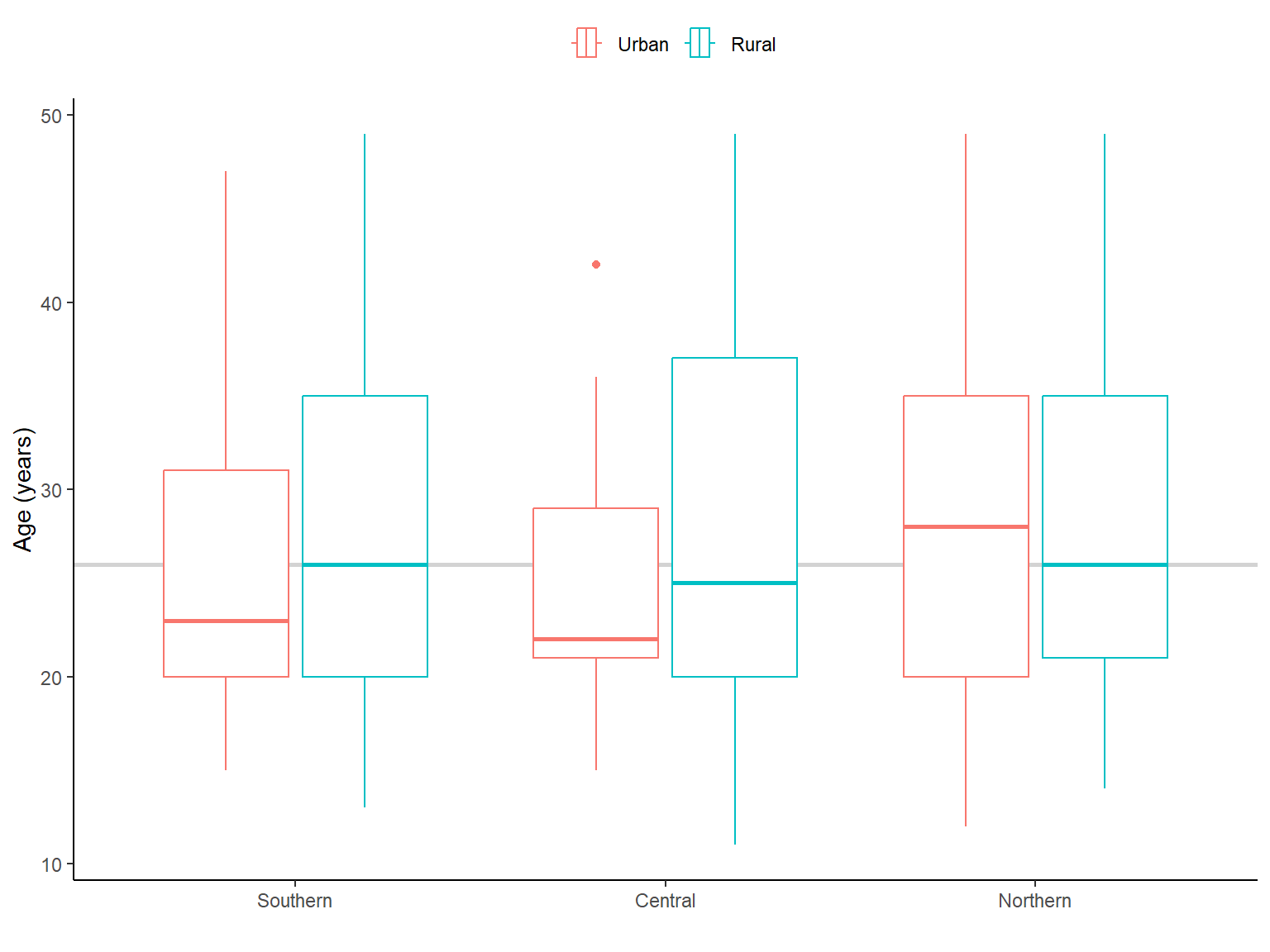
In addition, mean (and median) were higher in the northern region compared with southern and central regions (Figure 2.1). Whereas, mean/median age were higher in rural areas. We applied survey weights when calculating them.

Code

# Boxplot: Age per region and residency----
var_x <- "AGE_IN_YEARS"
x_label <- "Age (years)"

Malawi_WRA %>% 
  mutate(region = forcats::fct_relevel(region,"3", "2", "1")) %>% 
  ggplot(aes(x = !!sym(var_x), weight=wt, region, colour=urbanity)) +
  geom_vline(xintercept = median(Malawi_WRA$AGE_IN_YEARS), col = "lightgrey", size = 1) +
  geom_boxplot() + 
    scale_colour_manual("", values = col_break, labels = lab_reside)+
  #  geom_violin() + 
    coord_flip() +
  scale_y_discrete(label = lab_region) +
  theme_classic() +
  labs(y = "",
       x = x_label) +
  theme(legend.position = "top")

Figure 2.1: Age (in years) of women by residency and region in Malawi. The light grey line is the median age (years) for Malawi

2.1.2 Gender & Pregnancy

There is one entry labelled as “male” while the data set should only contain women, and there were 60 women pregnant or with unknown status, which were excluded from the data set.

Code

# Excluding the pregnant women and unknown status
Malawi_WRA  <- subset(Malawi_WRA, is_pregnant==0 | is.na(is_pregnant))

2.1.3 Malaria test

We needed to recode other values than positive/ negative into NA, also we did not follow the recode manual (we are not putting 0 for negative, but keeping 2).

Code

# Recoding others values into NA 
Malawi_WRA$Malaria_test_result <- ifelse(Malawi_WRA$Malaria_test_result==4| 
                                        Malawi_WRA$Malaria_test_result==6, 
                                         NA, Malawi_WRA$Malaria_test_result)

Malawi_WRA$Malaria_test_result  <- as.factor(Malawi_WRA$Malaria_test_result)

This variable has 22 missing values which would reduce the sample size. Hence, we need to evaluate whether the information provided would influence the results to decided whether to include this variable into the final model.

Can we identify if malaria is influencing Se status? - In ?fig-XX, we can see the plasma Se concentration by malaria test result, and it didn’t seem to have many differences between positive and negative malaria test, but maybe due to the high number of negative tests (see Section 2.1.8).

We could run the model with and without the variable and see if there is any difference in the final results.

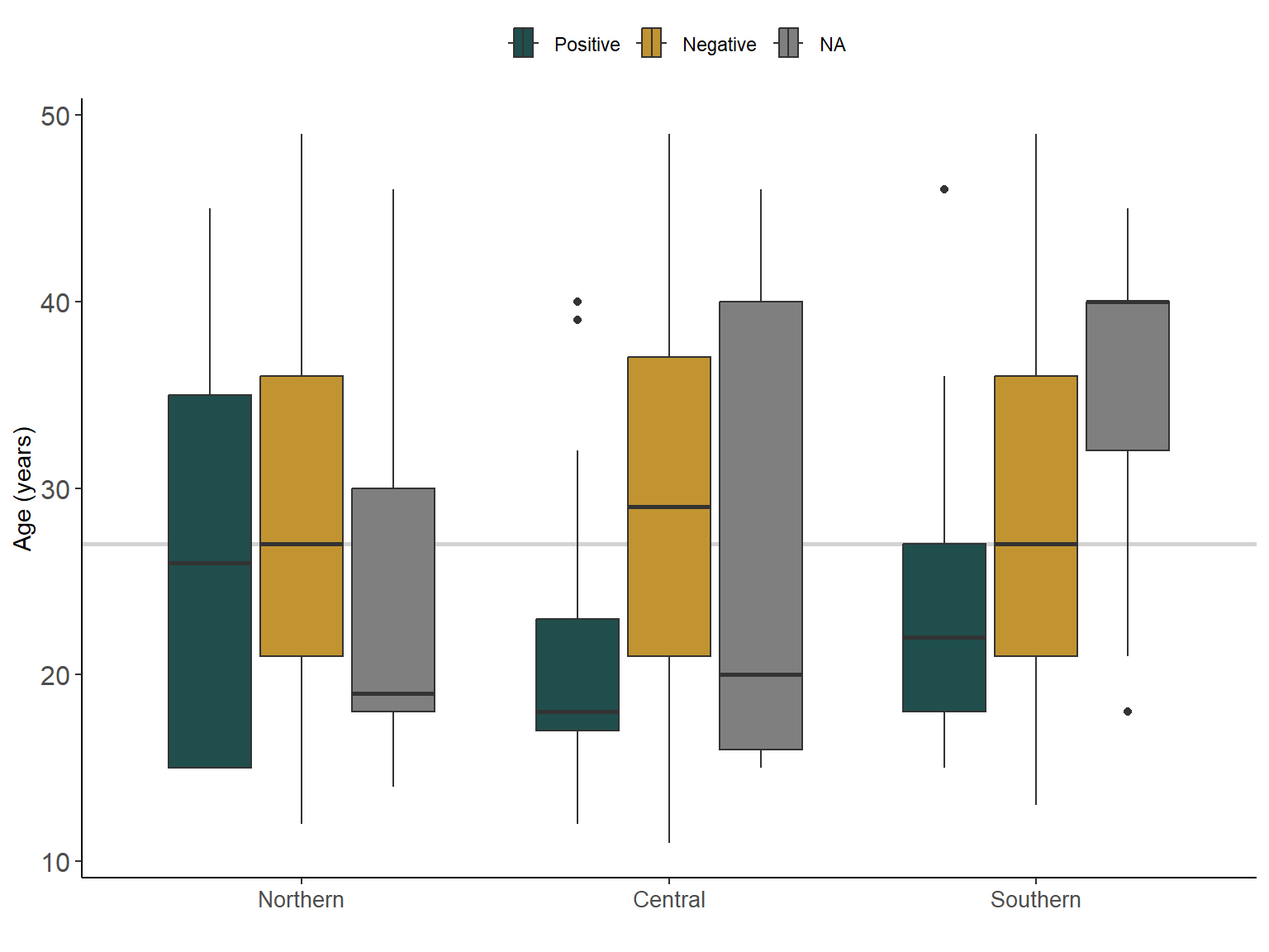
Interestingly, younger women tented to test positive to malaria in central and southern regions, as shown in Figure 2.2, which may be producing a confounding effect between age/malaria test and Se status.

Differences in the prevalence of malaria by age in WRA in Malawi were reported in the Micronutrient DHS report (REF).

Code

## Age per malaria test and residency ----
var_x <- "AGE_IN_YEARS"
x_label <- "Age (years)"
var_col <- "Malaria_test_result"
col_lab <- lab_malaria

value_median <- median(Malawi_WRA$AGE_IN_YEARS)

Malawi_WRA %>% 
  ggplot(aes(x = !!sym(var_x), weight=wt, # w/ survey weights
             region, fill=!!sym(var_col))) +
  geom_vline(xintercept = value_median, col = "lightgrey", size = 1) +
  geom_boxplot() + 
   scale_fill_manual("", values = col_binary, labels = col_lab)+
    coord_flip() +
  scale_y_discrete(label = lab_region) +
  theme_classic() +
  labs(y = "",
       x = x_label) +
  theme(legend.position = "top") +
  theme(strip.text = element_text(size = 12),
        axis.text.y = element_text(size = 12), 
        axis.text.x = element_text(size = 10))

Figure 2.2: Age (in years) of women by malaria test and region in Malawi. The light grey line is the median age (years) for Malawi

2.1.4 Supplementation

Similarly, as with the Malaria test, we found high number of missing values which would reduce the sample size by 28, and also only few reported consuming supplement (n=13), thus, we decided to exclude this variable.

2.1.5 Height & Weight

Missing values were coded as “999” for height and weight, we recoded to NA, according to the DHS documentation and recode standards reported in (ICF. 2018. Demographic and Health Surveys Standard Recode Manual for DHS7. The Demographic and Health Surveys Program. Rockville, Maryland, U.S.A.: ICF).

Code

# Height: Missing values (999 to NA)
Malawi_WRA$HEIGHT[Malawi_WRA$HEIGHT >999] <- NA

# Weight: Missing values (999 to NA)
Malawi_WRA$WEIGHT[Malawi_WRA$WEIGHT >999] <- NA

Height: The height distribution was normal with two potential outliers (i.e., one woman with a recorded height of 100.2), after recoding the missing values.
Weight: Some outliers were found as well, some weights were higher than expected, on the lower bound seems plausible given age and height.

2.1.6 Body Mass Index

We calculated the Body Mass Index (BMI) as it would be added to the model as a proxy for total food consumption.

We hypothesised that women with higher food intake may have higher plasma Se due to higher overall dietary Se intake. For instance, a normal BMI range (i.e., 18.5-24.9 kg/\(m^2\)) would likely mean that the food intake was providing enough food (i.e, energy) to maintain a normal body weight.

In Malawi, main source of energy (and some micronutrient) is maize, as it is the main staple crop which supplies more than 60% of the total energy supply (REF-Joy et al, , REF). Hence, we are exploring the BMI as a potential proxy of difference in plasma Se concentration due to differences in maize total consumption.

Code

# Creating BMI variable
Malawi_WRA$BMI<- Malawi_WRA$WEIGHT/(Malawi_WRA$HEIGHT/100)^2

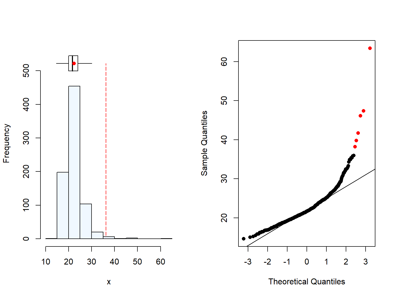
As expected, BMI also has some outliers due to the high weight of some women (Figure 2.3). We are not removing those values as the BMI is still plausible.

Code

summaplot(Malawi_WRA$BMI)

[1] 17  missing value(s) removed

Code

# Changing implausible to NA

Malawi_WRA$BMI[Malawi_WRA$BMI>300] <- NA

Figure 2.3: Distrubution of Body Mass Index (BMI) (kg/m^2) of women in Malawi

We could see that the northern region has overall higher BMI. This differences were only moderately significant when comparing the northern and the central region. Similar trend was found when we evaluated the wealth quintiles (Section 2.2.1), where the Northern region in Malawi has higher BMI & wealth quintile than the other two regions. This is unsurprising, as we can assume that BMI and wealth may be related, and it has been reported previously higher body weight in wealthier women in Malawi and in the region (REF, REF, REF).

There was a significant difference in the BMI between rural and urban women however, the number of urban were very low. Moreover, when we checked the results by region, the differences were only seeing for the southern region. These results should be interpret with care due to the difference in sample size between rural and urban.

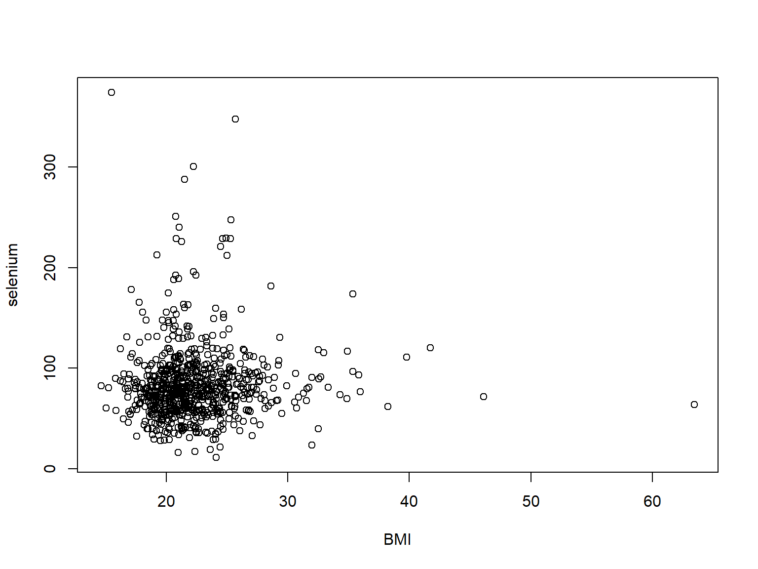
Moreover, as it can see in the scatter plot (Figure 2.4) and in the histogram, most of the population included in the study were within normal BMI range, and plasma Se concentration was not particularly influenced by BMI.

Code

# Scatter plot 
plot(selenium ~ BMI, Malawi_WRA)

Figure 2.4: Scatter plot showing relationship between plasma Se concentration and BMI in women of reproductive age in Malawi.

2.1.7 Selenium

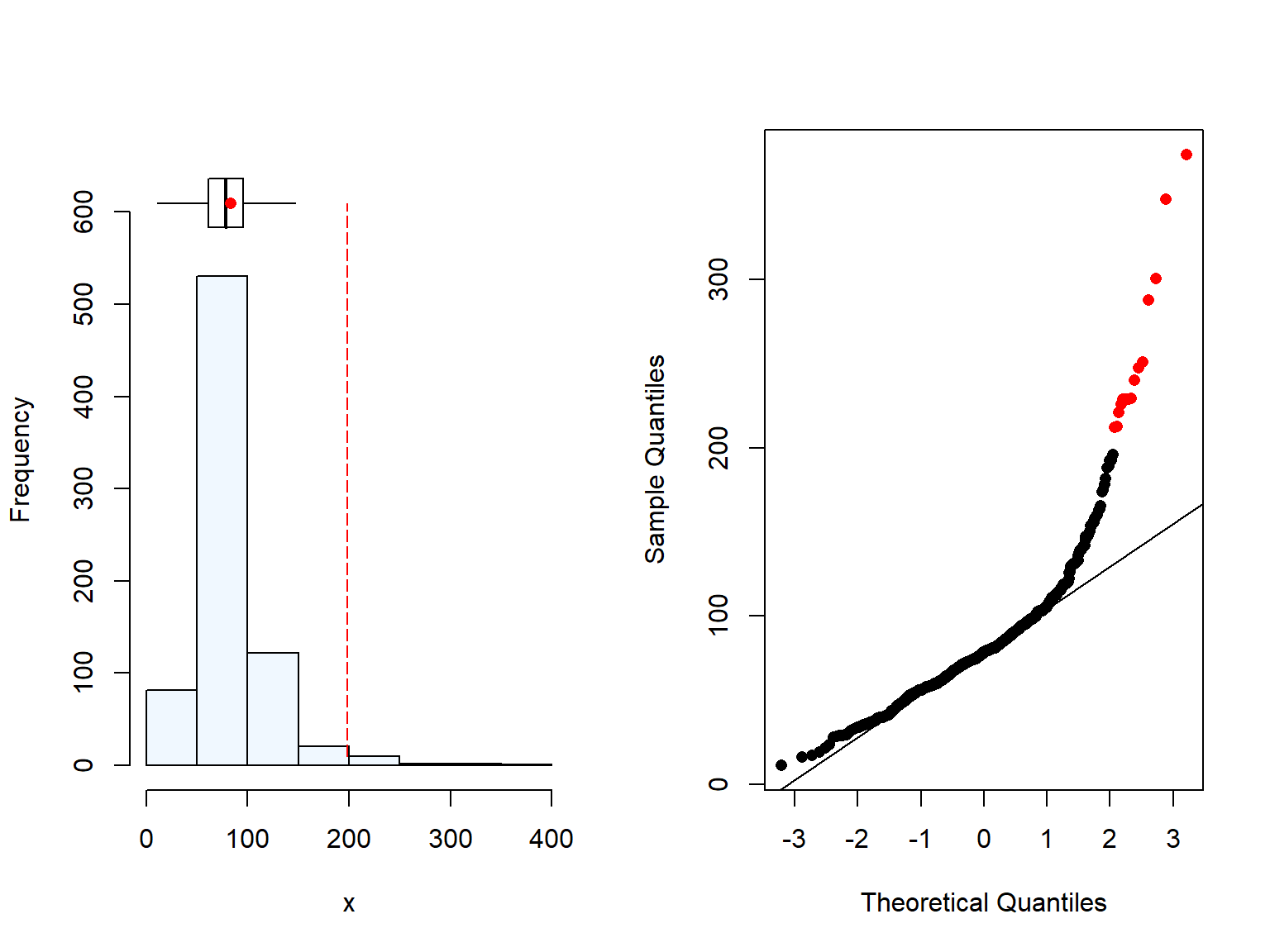
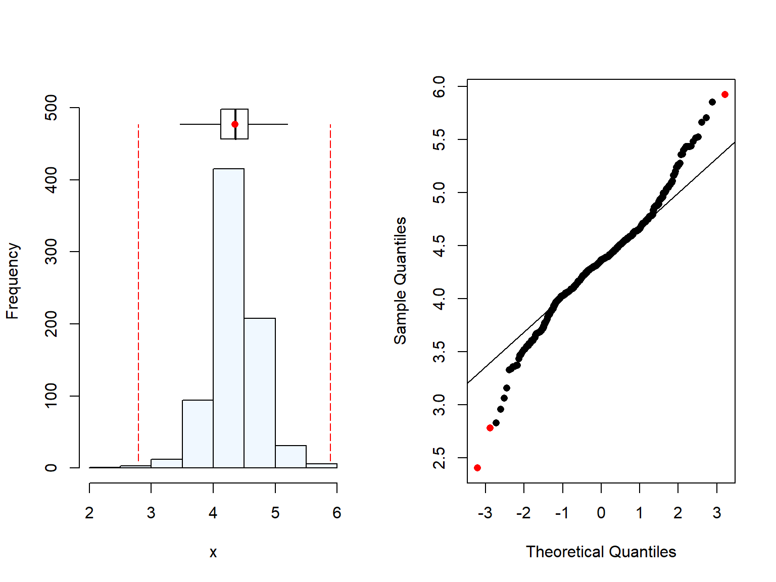
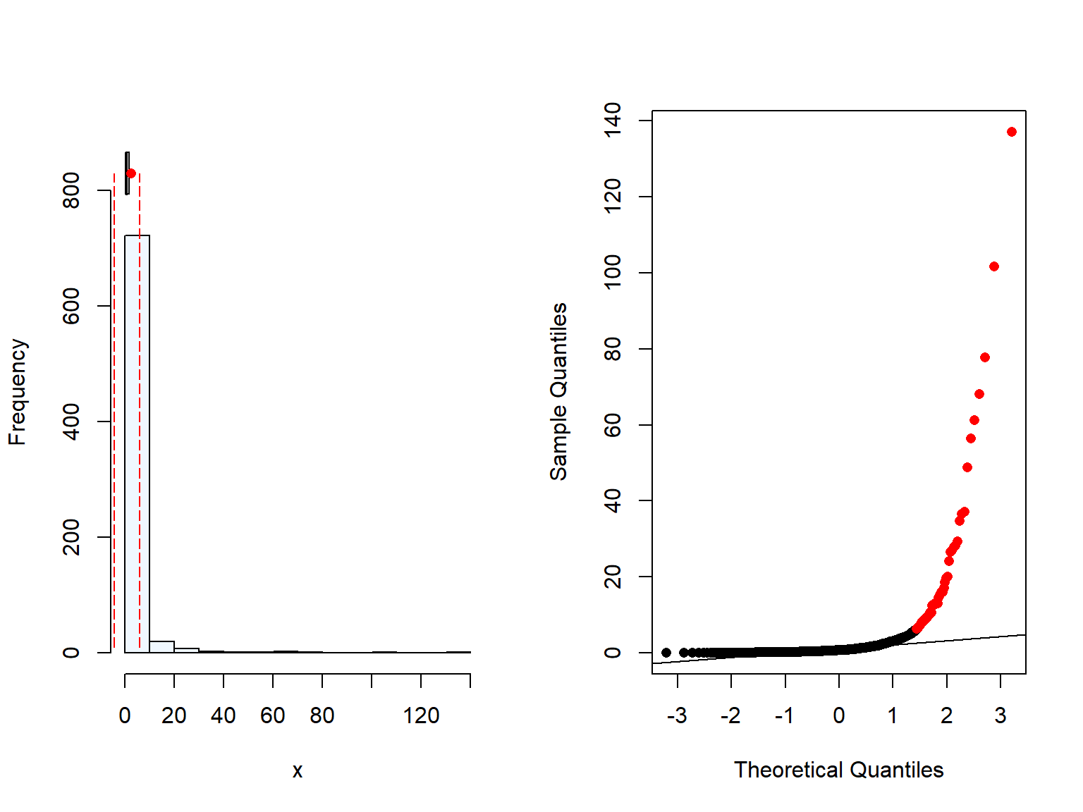
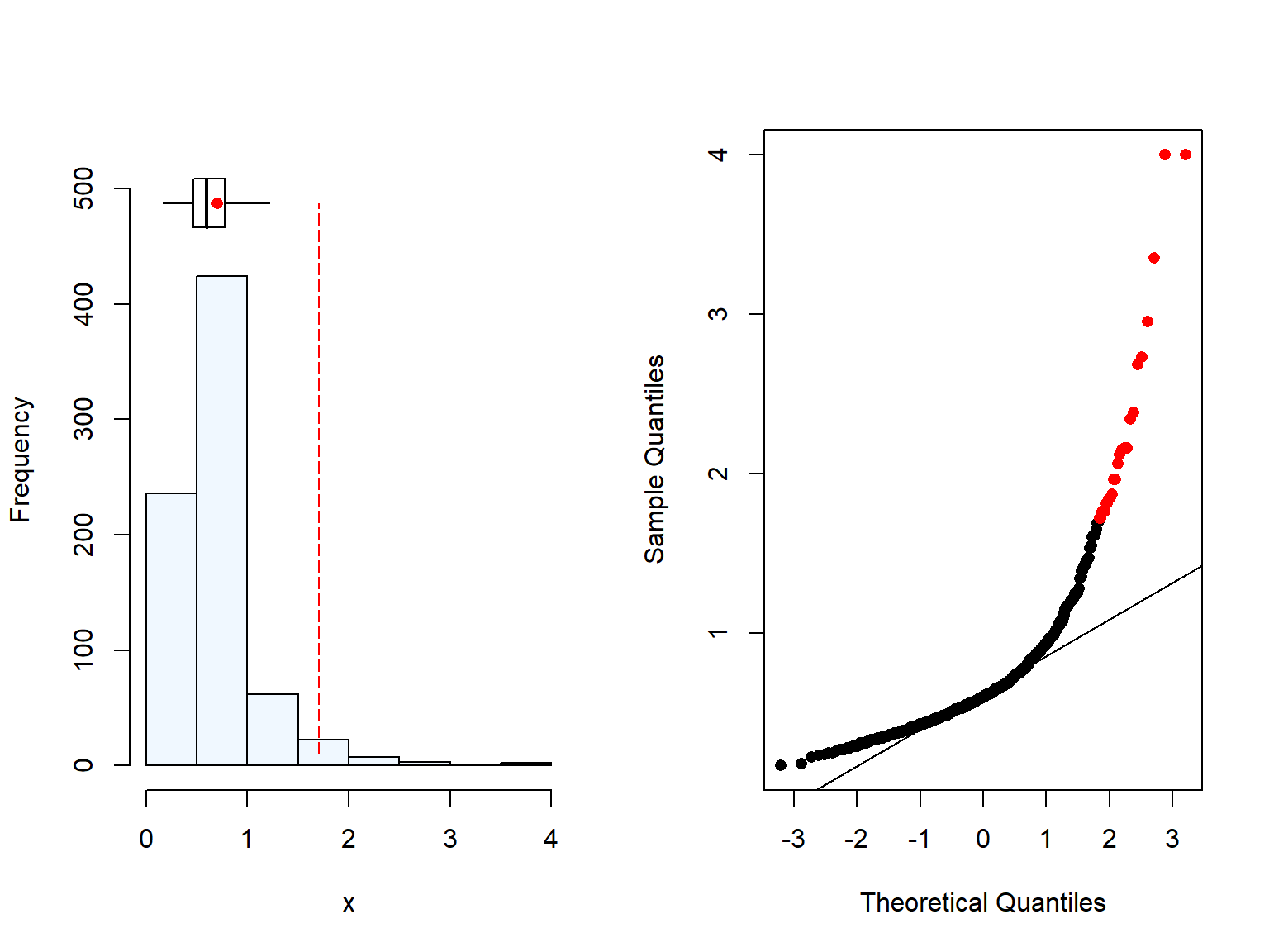
Plasma Se concentration is highly skewered, but when log-transformed it shows normality.

Code

# Distribution of plasma Se conc.
summaplot(Malawi_WRA$selenium)

[1] 34  missing value(s) removed

Code

# Distribution of log-transformend plasma Se conc.
summaplot(log(Malawi_WRA$selenium))

[1] 34  missing value(s) removed

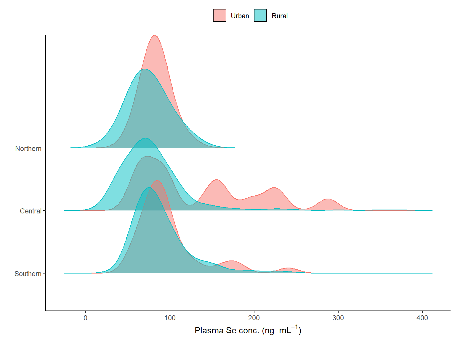
Moreover, when we see the distribution by region and residency, we can see that there are differences by regions (see Figure 2.5).

Code

# Ridges: Plasma Se per region and residency
# Selecting the variable & the label
var_x <- "selenium"
x_label <- plasma_lab
  
Malawi_WRA %>% filter(!is.na(!!sym(var_x))) %>% 
  mutate(region = forcats::fct_relevel(region,"3", "2", "1")) %>% 
  ggplot(aes(x = !!sym(var_x),  region, fill=urbanity, colour = urbanity)) +
  ggridges::geom_density_ridges(alpha = 0.5)  +
    scale_fill_manual("", values = col_break, labels = lab_reside)+
  scale_colour_discrete( guide = "none") +
  scale_y_discrete(label = lab_region) +
  theme_classic() +
  labs(y = "",
       x = x_label) +
  theme(legend.position = "top")

Figure 2.5: Distribution of the plasma Se concentration (ng/mL) of women in Malawi by region and the colour represents the urbanicity (no survey weights applied).

Plasma Se median values were higher in urban settings than in rural, and the highest in the Southern region.

Code

# Se Weighted mean/median by region
ddply(Malawi_WRA,~region, summarise,median=matrixStats::weightedMedian(selenium, wt,na.rm = T))

  region   median
1      1 73.68868
2      2 71.07763
3      3 80.76456

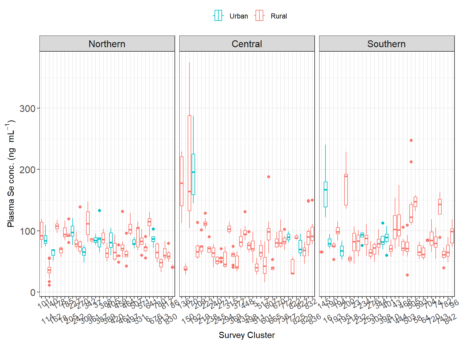
Then, the median disaggregated by region and residency showed that Northern and Southern urban population had the highest plasma Se median concentration, while the Central region were the lowest, particularly for women living in rural settings as shown in Figure 2.6.

Code

# Se Weighted median by region & urbanity
ddply(Malawi_WRA,.(region, urbanity), summarise,median=matrixStats::weightedMedian(selenium, wt,na.rm = T))

  region urbanity   median
1      1        1 83.75346
2      1        2 72.22663
3      2        1 95.31994
4      2        2 69.82099
5      3        1 81.09410
6      3        2 80.66016

Interestingly, while the women in the Northern-urban areas had higher plasma Se than their southern counterpart, the women in the Southern-rural areas had higher plasma Se those in Northern-rural areas.

In addition, women who live in urban setting of the Central region had similar plasma Se median concentration as women in the northern region in rural settings.

Code

data.df <- Malawi_WRA %>% dplyr::filter(!is.na(selenium))

data.df$survey_cluster1 <- as.character(data.df$survey_cluster1)
data.df$urbanity <- as.factor(data.df$urbanity)

 # Custom legend colour & labels
 col_break <- c("1" = "#00BFC4", "2" = "#F8766D")
 col_labels <- c("1" = "Urban", "2" = "Rural")
 unit_micro <- expression(paste("Plasma Se conc. (ng  ",  mL^{-1}, ")"))
 
micro_region(data.df, micro = selenium, var_sorting = survey_cluster1,
             var_colouring = urbanity, unit_micro = unit_micro, label_sorting = "Survey Cluster", 
             col_break =col_break, col_labels = col_labels)

# Custom X-axis labels 
col_labels <- c("Urban", "Rural")

Figure 2.6: Variation in plasma Se concentration (ng/mL) of women in Malawi by cluster. Information is divided by region and colour represents the urbanicity.

2.1.8 Inflammation

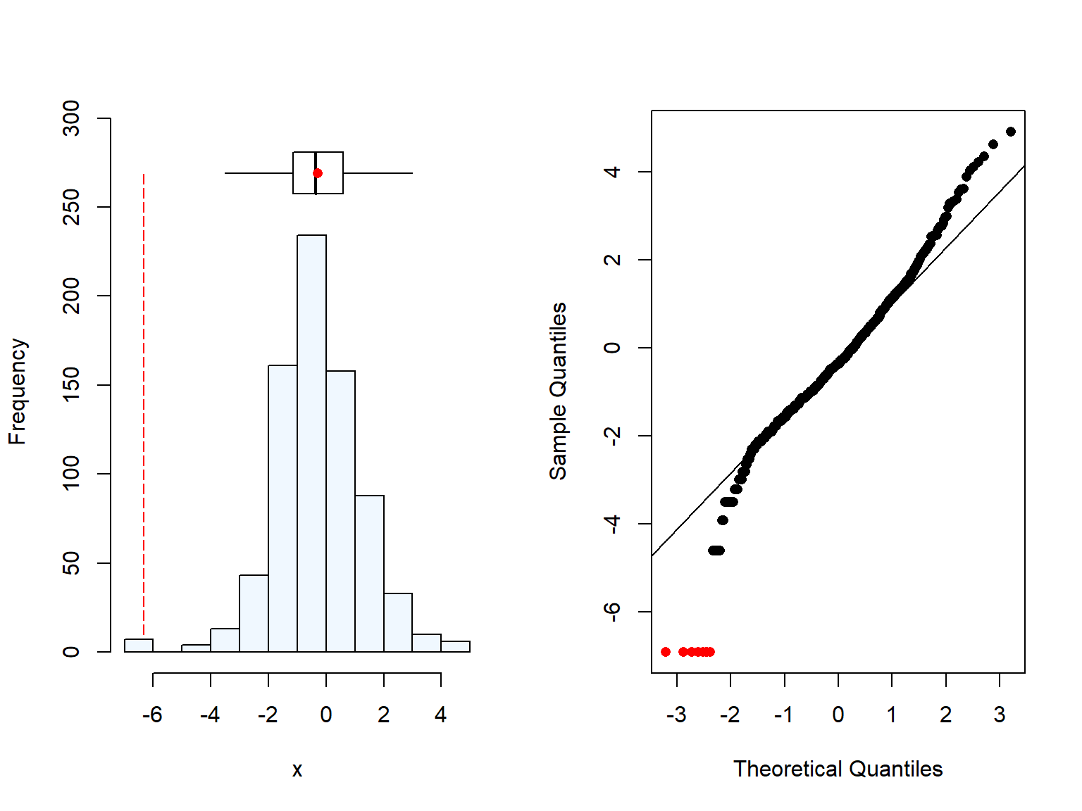
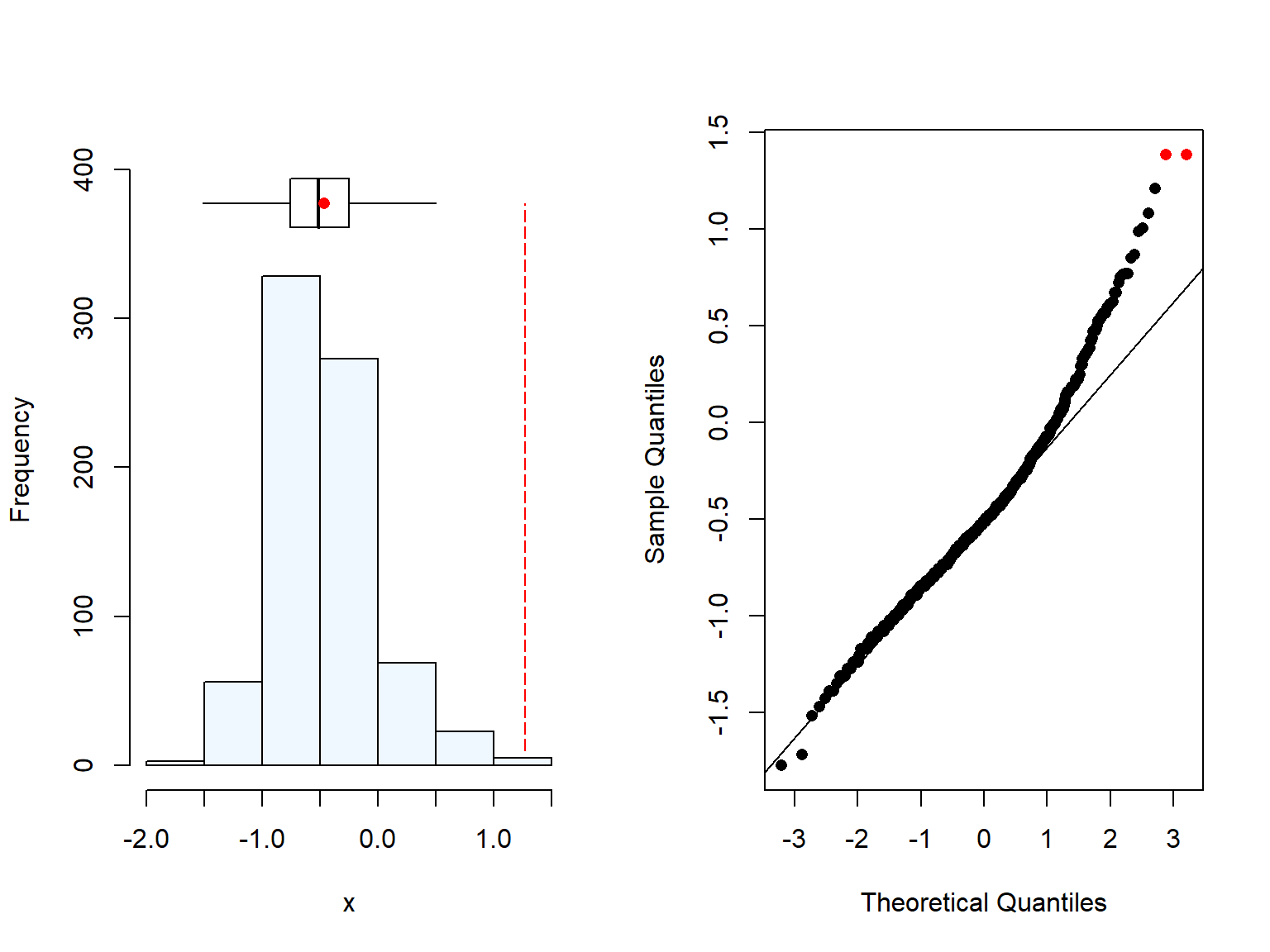
Both CRP () and AGP () were measured in women, of which we had 13 and 13 missing values respectively. We can also see that both variables were skewered and hence, we needed to log-transform them, which turned them into normality.

Code

# Normality check
summaplot(data.df$crp)

[1] 13  missing value(s) removed

Code

summaplot(data.df$agp)

[1] 13  missing value(s) removed

Code

# Normality check, after log-transformation
summaplot(log(data.df$crp))

[1] 13  missing value(s) removed

Code

summaplot(log(data.df$agp))

[1] 13  missing value(s) removed

Then, we checked values that were high (inflammation cut-offs: CRP > 5 mg/L and/or AGP > 1 g/L, REF-BRINDA, REF-DHS docu). From the total sample, after excluding women who were missing plasma Se concentration, only 69 women and 97 had CRP and AGP values that indicate inflammation. According to the 2015-2016 MDHS report, inflammation was reported around 12% but it was consistent across age groups, residency, and wealth quintiles.

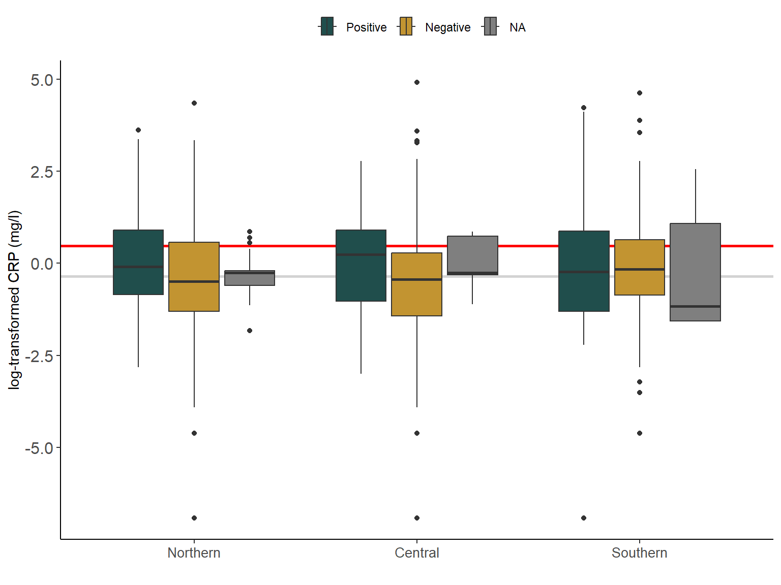
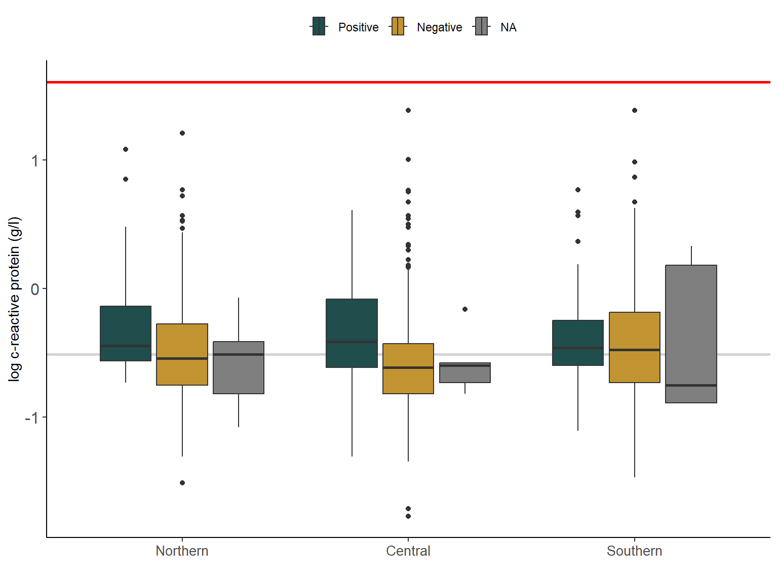
However, when we look at the CRP and AGP values by region, we can see in Figure 2.7 and ?fig-2_6b that CRP and AGP values were higher among those women who reported positive malaria tests. Interestingly, values in the southern region of Malawi were similarly high for both positive and negative malaria tests. This could be linked to the higher prevalence of other (infectious) diseases such as HIV.

It could be that this variable is correlated with Malaria, hence by including these two inflammation variables, we may be accounting for the potential influence of the malaria in the plasma Se.

(AGP: 0.54 g/L and CRP: 0.16 mg/L, see Lou et al paper (BRINDA adjustement)

However, malaria prevalence was higher in rural areas and for the different wealth quintiles (WQ), with lowest WQ being 6-times higher than the highest WQ. Since, these two variables may influence Plasma Se status we are including it in the model.

Code

## CRP per malaria test and residency ----
var_x <- "crp"
x_label <- "log-transformed CRP (mg/l)"
cut_off <- log(5) #crp
var_col <- "Malaria_test_result"
col_lab <- lab_malaria

value_median <- log(median(pull(Malawi_WRA[,var_x]), na.rm = TRUE))

Malawi_WRA %>% 
  ggplot(aes(x = log(!!sym(var_x)), weight=wt, # w/ survey weights
             region, fill=!!sym(var_col))) +
  # CRP median (log-transformed) values
  geom_vline(xintercept = value_median, col = "lightgrey", size = 1) +
  # CRP cut off values for inflammation
  geom_vline(xintercept = log(cut_off), col = "red", size = 1) +
  geom_boxplot() + 
     scale_fill_manual("", values = col_binary, labels = col_lab)+
    coord_flip() +
  scale_y_discrete(label = lab_region) +
  theme_classic() +
  labs(y = "",
       x = x_label) +
  theme(legend.position = "top") +
  theme(strip.text = element_text(size = 12),
        axis.text.y = element_text(size = 12), 
        axis.text.x = element_text(size = 10))

Figure 2.7: Variation in c-reactive protein (CRP) (mg/L) (log-transformed) of women in Malawi by region and malaria test resutls. Grey line is the median CRP (log-transformed). Red line is the log-tranformed CRP cut-off value for infammation (5mg/L).

Code

## AGP per malaria test and residency ----
var_x <- "agp"
x_label <- "log-transformed AGP (g/l)"
x_label <- "log c-reactive protein (g/l)"
cut_off <- log(1) #AGP
var_col <- "Malaria_test_result"
col_lab <- lab_malaria

value_median <- log(median(pull(Malawi_WRA[,var_x]), na.rm = TRUE))

Malawi_WRA %>% 
  ggplot(aes(x = log(!!sym(var_x)), weight=wt, # w/ survey weights
             region, fill=!!sym(var_col))) +
  geom_vline(xintercept = value_median, col = "lightgrey", size = 1) +
  geom_vline(xintercept = log(5), col = "red", size = 1) +
  geom_boxplot() + 
     scale_fill_manual("", values = col_binary, labels = col_lab)+
    coord_flip() +
  scale_y_discrete(label = lab_region) +
  theme_classic() +
  labs(y = "",
       x = x_label) +
  theme(legend.position = "top") +
  theme(strip.text = element_text(size = 12),
        axis.text.y = element_text(size = 12), 
        axis.text.x = element_text(size = 10))

Figure 2.8: Variation in (AGP) (g/L) (log-transformed) of women in Malawi by region and malaria test resutls. Grey line is the median AGP (log-transformed). Red line is the log-tranformed AGP cut-off value for infammation (1mg/L).

2.2 Socio-economic data (DHSDATA)

There were some variables that may be related to differences in individual plasma Se variations that were recorded in the household questionnaire, for instance whelath quintile and wealth index.

Code

# Loading Wealth index and other variables (00_cleaning-dhs, line 346)
dhs.df<- haven::read_dta(here::here("data","MWIR7AFL.dta")) # survey data DHS

We extracted the socio-economic information from the DHS survey, however, we are only interested in the data for women and those with reported Plasma Se values.

Code

# Renaming and selecting variables of interest (reducing the number of variables)

dhs.df <- dhs.df %>% dplyr::rename( 
  survey_cluster1='v001',
  household_id1='v002',
  LINENUMBER='v003', 
  survey_strata= "v022",
  PSU = "v021", 
  region = 'v101', 
  urbanity = "v102", 
  # region = 'v024', 
  age_year = "v012", # for consistency 
  wealth_quintile= "v190",
  wealth_idx= "v190a", # to check for wealth missing values
  Literacy= "v155",
  education_level= "v106", 
  source_water = "v113", # source of drinking water
  # person_id=WomenID,
  is_lactating= "v404", # breastfeeding yes=1, no=0
  is_smoker= "v463a" # Only cover cigarettes (other smoking variables)
) 
  
DHSDATA <- dhs.df %>% dplyr::select(survey_cluster1, household_id1, LINENUMBER, survey_strata, PSU,
             region, urbanity,  age_year, wealth_quintile, wealth_idx, Literacy,
             education_level, source_water, is_lactating, is_smoker, sdist) %>% 
  mutate_at(c("region", "urbanity", "wealth_quintile", "wealth_idx", "education_level"  ,"source_water"), as.factor)

# New variable with district names
DHSDATA$dist_name <- haven::as_factor(DHSDATA$sdist) 
DHSDATA$sdist  <- as.factor(DHSDATA$sdist)

2.2.1 Wealth Quintiles

Code

# Wealth quintile
class(DHSDATA$wealth_quintile)
sum(is.na(DHSDATA$wealth_quintile))
table(DHSDATA$wealth_quintile)
DHSDATA$wealth_quintile  <- as.factor(DHSDATA$wealth_quintile)

Wealth index is calculated at household level, and it is based on the goods and housing characteristics. It was assessed using Principle Component Analysis and then made to each quintile to represent 20% of the population. In the report published by the NSO (2017), they reported significant differences between the number of individuals in each WQ when disaggregated by rural/urban residency.

When plotted the WQ per region, we can see that the Central and Southern region have more or less even distribution of the WQ, however the Northern region has predominately highest and higher WQ, accounting for more than 60% of the population in the Northern region (unweighted results).

Code

# Wealth index (by urban/rural)
class(DHSDATA$wealth_idx)
sum(is.na(DHSDATA$wealth_idx))
table(DHSDATA$wealth_idx)
DHSDATA$wealth_idx  <- as.factor(DHSDATA$wealth_idx)

Then, there is another wealth variable (wealth_idx) that it is disaggregated by residency (rural/urban). This was developed recently in response of some criticism over the way the index is calculated, for more information see (REf=).

2.2.2 Education

Code

# Education
class(DHSDATA$education_level)
sum(is.na(DHSDATA$education_level))
table(DHSDATA$education_level)
haven::print_labels(DHSDATA$education_level)
DHSDATA$education_level  <- as.factor(DHSDATA$education_level)

We could see when wealth and education were plotted together, that most of the people with higher education was in the highest wealth quintile which is in line with the NSO report (NSO, 2017). Similarly, women in the lowest WQ has no high education.

All education and wealth level have representation in all three regions. Again, when looking at the data we could see that there is a slight “over-reporting” of the wealthiest quintiles.

Hence, we excluded this variable as it could possibly be confounding effect.

Code

# Wealth quintile 1-5 (lowest to highest)
# Education 0-3 (low to high)

plot(DHSDATA$wealth_quintile, DHSDATA$education_level, 
     main="Wealth vs Education",
     xlab="Wealth Q", ylab="Education level", pch=19)

Similarly, when we plotted the Education by region, we could see the same trend as in the WQ.

2.2.3 Literacy

This variable was excluded as some of the results were misaligned. For instance, when comparing the literacy with the education level, all the women with secondary education reported literacy (n = NA), however, there were women who reported no literacy (0), but secondary education (2).

2.2.4 Source of water

The source of water could have an influence on the plasma Se concentration, specially if the water is coming from local underground water or ponds, as the concentration of drinking Se water may be different according to their location, while drinking water coming from water bottled may have no minerals on it.

Code

# source of drinking water 
class(DHSDATA$source_water)
table(DHSDATA$source_water)
haven::print_labels(DHSDATA$source_water)

# New variable with descriptions
DHSDATA$source_water_ds <- haven::as_factor(DHSDATA$source_water)

2.3 Combining DHS datasets: Plasma Se & covariates

Code

# Merging with DHS dataset to obtain Wealth index and other variables

EligibleDHS <- Malawi_WRA %>% 
 left_join(., DHSDATA %>% 
          dplyr::select(survey_cluster1, household_id1, LINENUMBER, 
                 wealth_quintile, wealth_idx, Literacy, education_level, 
            source_water, is_lactating, is_smoker, sdist, 
            dist_name))

According to the study of Phiri et al (2019), the influencing factors for Plasma Se (for WRA) in Malawi were soil type and proximity to Lake Malawi.

In addition, other authors have reported that socio-economic characteristics may influence Se status.

Here we are exploring the variability of Plasma Se according to those variables. First within the same dataset.

2.3.1 Wealth & Plasma Se

After merging the datasets, some WQ were missing, hence following recommendations form F.S we used the household WQ for those available to impute it. They were available for 17 of the 39 observation with missing values. For Plasma Se, we only have values for 770.

2.3.1.1 Data inputation: Wealth quintile and index

First, we checked whether the missing information on wealth was the same for the two variables (Q and index).

Code

#Checking rows with missing value for wealth Q
n <- which(is.na(EligibleDHS$wealth_quintile))
#Checking rows with missing value for wealth Indx
m <- which(is.na(EligibleDHS$wealth_idx))
# Checkin that are the same 
table(n==m)


TRUE 
  29

Then, we identifed for which cases we could inpute the informationf from the household level dataset.

Code

# Identifying HH ID & cluster of missing socio-eco info
subset(EligibleDHS, is.na(EligibleDHS$wealth_quintile), 
       select = c("household_id1","survey_cluster1")) %>% left_join(.,DHSDATA) %>% 
  group_by(survey_cluster1, household_id1) %>% dplyr::count(wealth_quintile, wealth_idx, urbanity) %>% 
  filter(!is.na(wealth_quintile)) %>%
  knitr::kable()

survey_cluster1	household_id1	wealth_quintile	wealth_idx	urbanity	n
5	4	1	1	2	1
23	68	3	4	2	1
37	70	5	4	1	2
114	4	5	2	1	2
114	283	5	3	1	1
140	51	2	3	2	1
140	111	4	4	2	2
294	64	4	5	2	1
342	15	2	2	2	1
369	180	1	1	2	2
444	107	3	3	2	1
468	147	4	5	2	1
498	229	4	4	2	3
511	257	2	2	2	1
720	267	3	3	2	1

Then, we inputed the wealth Q and indx. from the cluster to the WRA dataset. By creating a dataframe with the information above, and looping over the missing values with information.

Code

#Sorting Wealth Q for each HH ID & cluster of missing info
Wealth <- subset(EligibleDHS, is.na(EligibleDHS$wealth_quintile), 
       select = c("household_id1","survey_cluster1")) %>% 
   left_join(., DHSDATA %>% 
             dplyr::select(c("household_id1","survey_cluster1", "wealth_quintile", "wealth_idx"))) %>% 
  group_by(survey_cluster1, household_id1) %>%
  filter(!is.na(wealth_quintile)) %>% 
  distinct()


# Generate a loop to assign Wealth Q from other member of the HH to non-reported people in biomarker survey data
for(i in seq_along(Wealth$household_id1)){
  
EligibleDHS$wealth_quintile[EligibleDHS$survey_cluster1 %in% Wealth$survey_cluster1[i] &
                              EligibleDHS$household_id1 %in% Wealth$household_id1[i]] <- Wealth$wealth_quintile[i]

EligibleDHS$wealth_idx[EligibleDHS$survey_cluster1 %in% Wealth$survey_cluster1[i] &
                              EligibleDHS$household_id1 %in% Wealth$household_id1[i]] <- Wealth$wealth_idx[i]
}

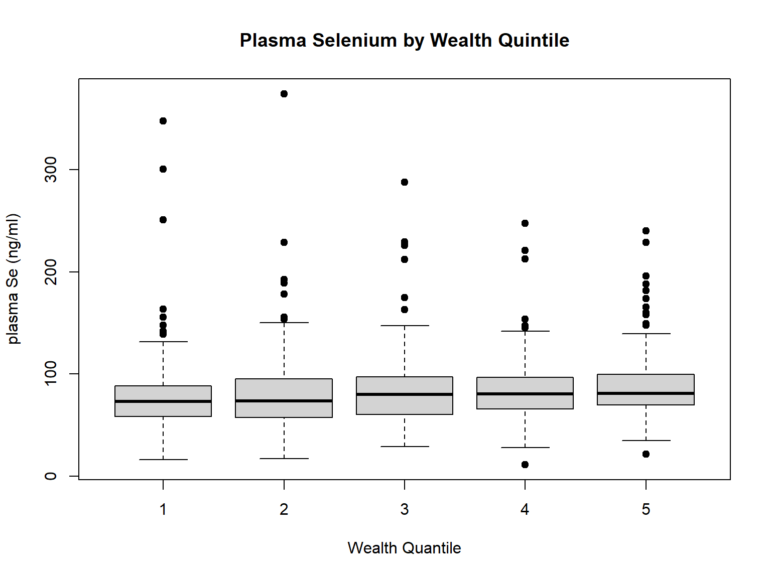
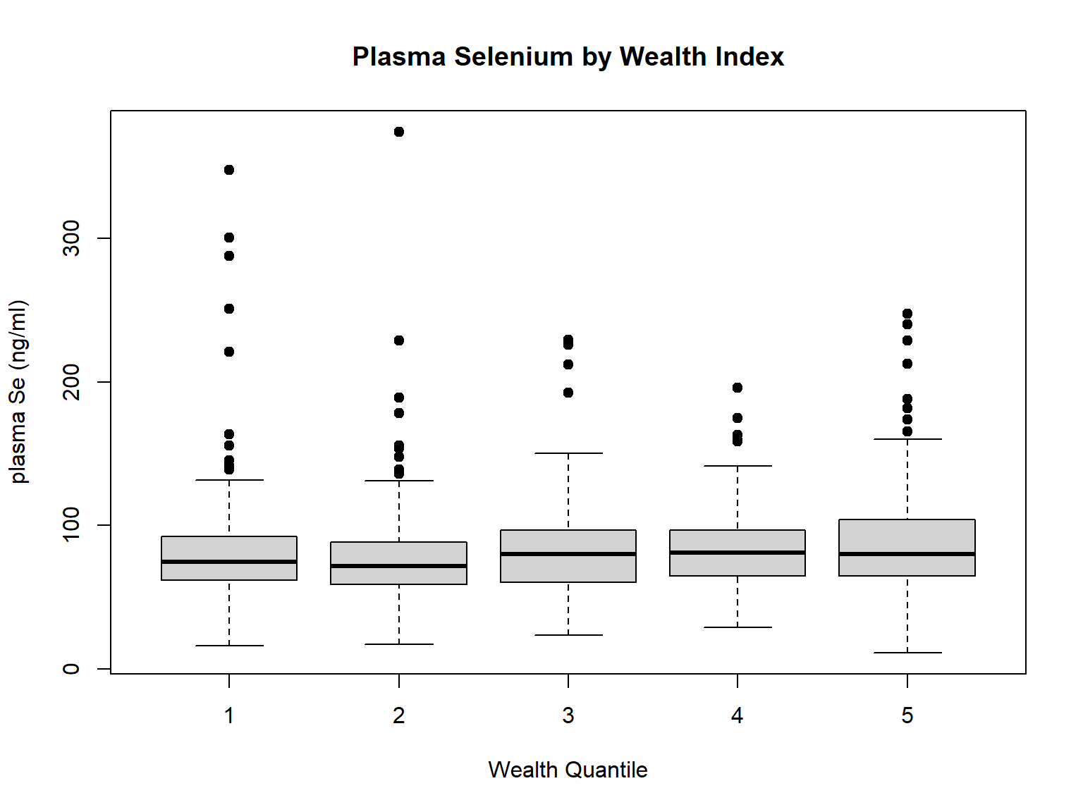
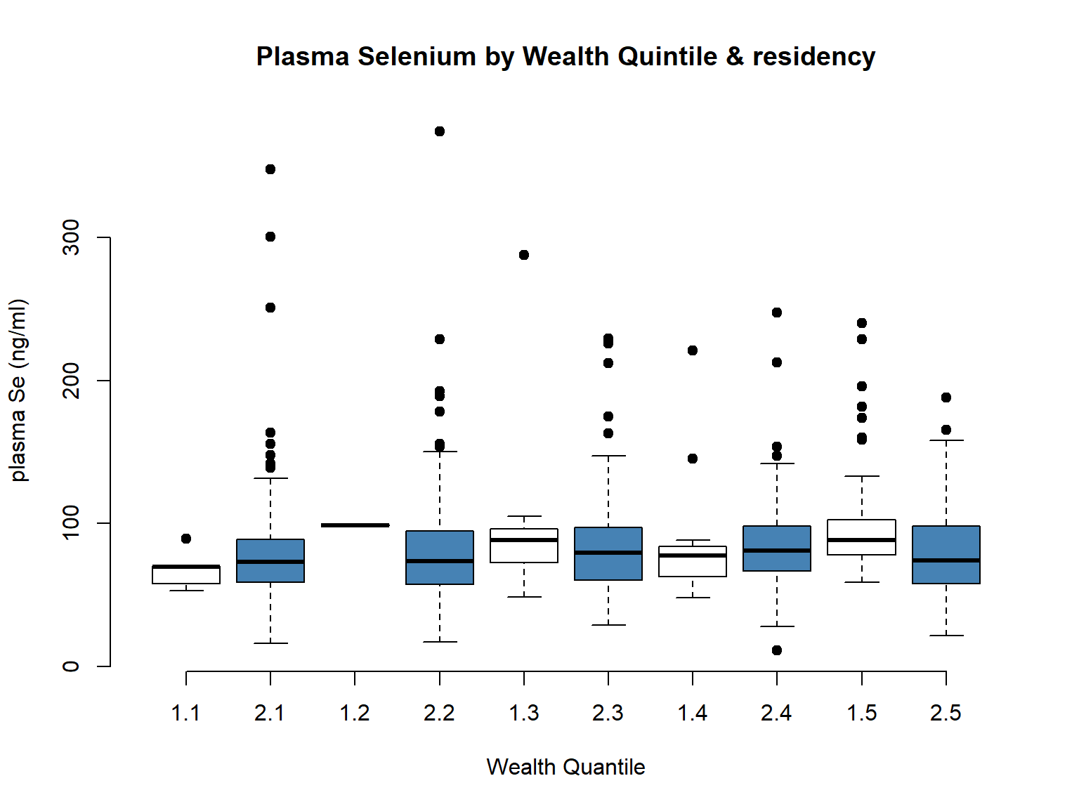
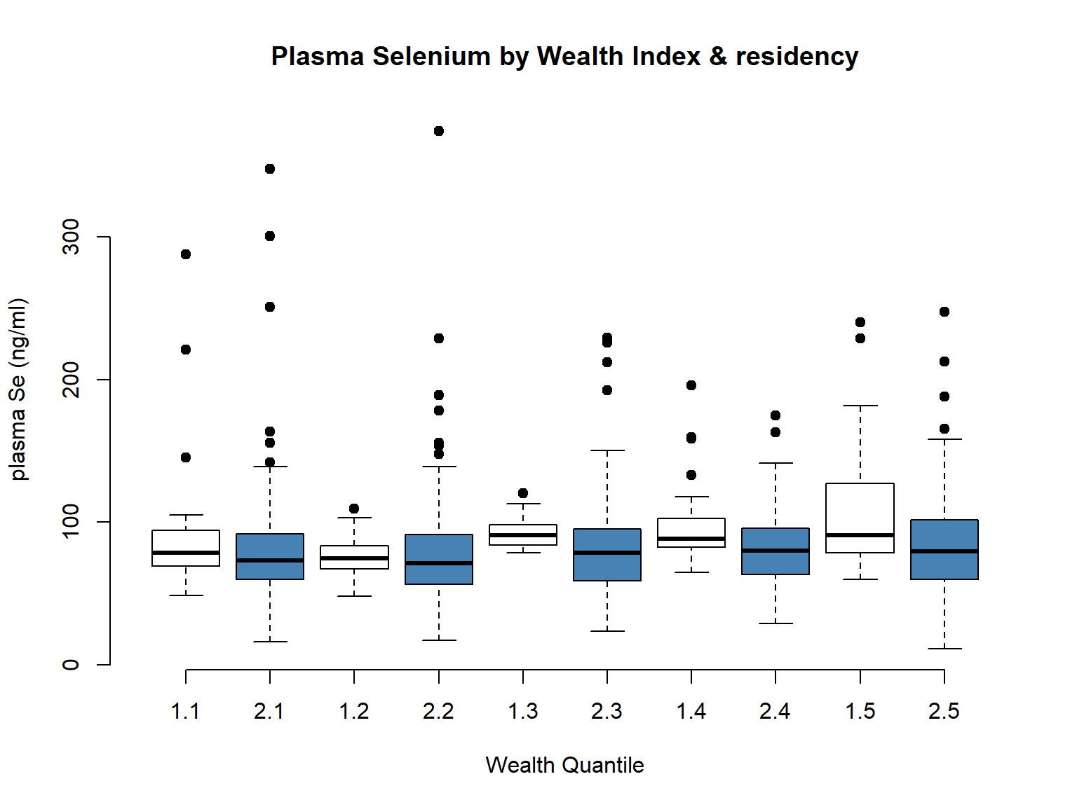
Then, we compared plasma Se concentration by the two wealth variables. We can see that there are no much differences (Fig.). However, when disaggregating the data by rural and urban, we could see differences in the trends (See Fig). Since we are modeling based on this urban/rural differences, we chosen to use the wealth_idx variable in our model.

Code

# Wealth Quintile
boxplot(selenium ~ wealth_quintile, data = EligibleDHS, 
     main="Plasma Selenium by Wealth Quintile",
     xlab="Wealth Quantile", ylab="plasma Se (ng/ml)", pch=19)

Code

# Wealth Idx
boxplot(selenium ~ wealth_idx, data = EligibleDHS, 
        main="Plasma Selenium by Wealth Index",
        xlab="Wealth Quantile", ylab="plasma Se (ng/ml)", pch=19)

Code

boxplot(selenium ~ urbanity*wealth_quintile, data = EligibleDHS, 
        main="Plasma Selenium by Wealth Quintile & residency",
        xlab="Wealth Quantile", ylab="plasma Se (ng/ml)", pch=19, 
        col = c("white", "steelblue"), frame = FALSE)

Code

boxplot(selenium ~ urbanity*wealth_idx, data = EligibleDHS, 
     main="Plasma Selenium by Wealth Index & residency",
     xlab="Wealth Quantile", ylab="plasma Se (ng/ml)", pch=19, 
     col = c("white", "steelblue"), frame = FALSE)

Finally, when we checked the overall distribution of the variable, seemed more sensible to use the combined (wealth_quintile) as the shape of the variable looked more equally distributed for our sample subset.

Wealth Quintile vs Wealth Index (urban/rural)
	1	2	1	2
1	5	141	28	121
2	1	144	33	126
3	12	145	18	115
4	20	158	21	150
5	86	79	24	155

2.3.2 Education level

Plasma Se values were slightly higher in the highest education level, with lower variability, while the opposite was true for the primary education level.

2.3.3 Place of residency

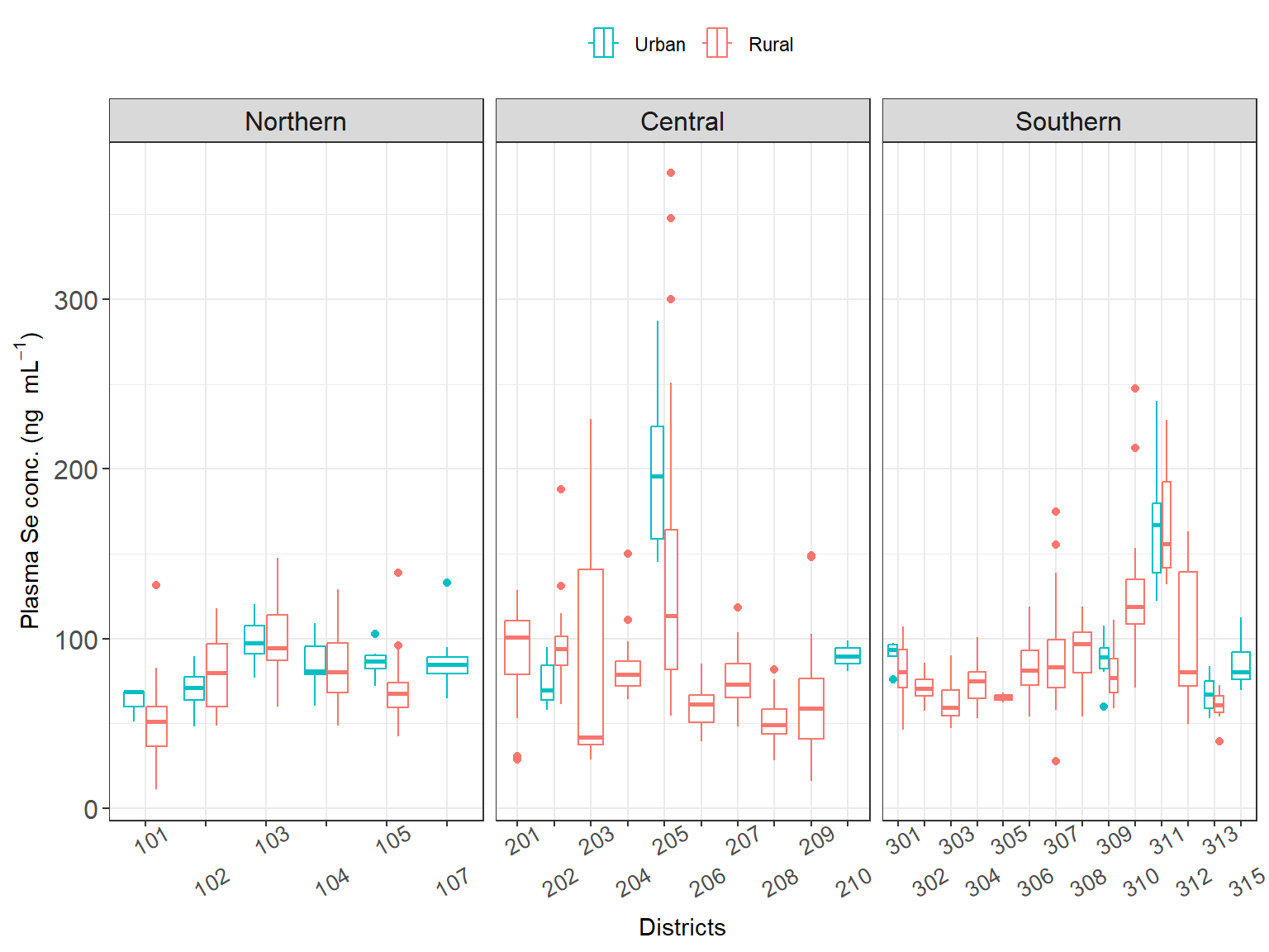
Plasma Se values were similar when aggregated by region, whereas we can start seeing some differences when we are plotting the results by district. Also notice, that the number of observations per district is 1) much smaller and 2) much diverse (from 0 to 51).

There are missing values 29 for the district variable which is an important variable (See Chapter 4), this was solved by using the district, of the same cluster (EA) as they should be in the same district.

Code

# Checking if we have same cluster with sdist for imputing.
test <- unique(EligibleDHS$survey_cluster1[is.na(EligibleDHS$sdist)])

EligibleDHS %>% filter(survey_cluster1 %in% test) %>% 
  distinct(survey_cluster1, sdist)

# A tibble: 48 × 2
   survey_cluster1 sdist
             <dbl> <fct>
 1             140 <NA> 
 2             114 <NA> 
 3             219 <NA> 
 4             369 <NA> 
 5              58 <NA> 
 6             294 <NA> 
 7             498 <NA> 
 8             468 <NA> 
 9             140 101  
10              37 107  
# ℹ 38 more rows

Code

# Fixing the missing values
for(i in 1:length(test)){
  
x <- unique(na.omit(EligibleDHS$sdist[EligibleDHS$survey_cluster1 %in% test[i]]))
EligibleDHS$sdist[EligibleDHS$survey_cluster1 %in% test[i]] <- x

x <- unique(na.omit(EligibleDHS$dist_name[EligibleDHS$survey_cluster1 %in% test[i]]))
EligibleDHS$dist_name[EligibleDHS$survey_cluster1 %in% test[i]] <- x
}

sum(is.na(EligibleDHS$sdist))

[1] 0

Because we are exploring how much Plasma Se variability is explained by Maize Se concentration, we do not need to apply (or worry about) the weights. Only, we would need to apply them if we want to express some findings at population level, e.g., perc. of population at risk. We are not likely to do that, as 1) it is not the objective of the study/ model, and 2) we are working at certain scales where data will not be representative (e.g., district).

Note: What it would be important to check, it is whether the data is balance (e.g., highly skewed to one side and hence driving the model outcomes). We checked wealth by region and it seemed that there is a slight unbalance for the lowest Q in the middle region and towards the highest Q in the Northern region. See above (Section 2.2.1). Maybe we need to check for confounding effect.

Code

 # Custom legend colour & labels
 col_break <- c("1" = "#00BFC4", "2" = "#F8766D")
 col_labels <- c("1" = "Urban", "2" = "Rural")
 unit_micro <- expression(paste("Plasma Se conc. (ng  ",  mL^{-1}, ")"))
 
micro_region(EligibleDHS, micro = selenium, var_sorting = sdist,
             var_colouring = urbanity, unit_micro = unit_micro, label_sorting = "Districts", 
             col_break =col_break, col_labels = col_labels)

Code

EligibleDHS %>% group_by(dist_name, region) %>% 
  summarise(Median_se = median(selenium, na.rm = TRUE)) %>% 
  arrange(desc(Median_se)) %>% knitr::kable()

dist_name	region	Median_se
ndanje	3	157.80285
salima	2	141.99920
chikwawa	3	118.81947
kasungu	2	100.68548
mulange	3	97.02449
nkhatabay	1	95.25494
nkhota kota	2	92.60358
lilongwe city	2	89.82441
mzuzu city	1	84.78483
phalombe	3	84.29541
thyolo	3	83.34044
mangochi	3	82.32660
mwanza	3	81.29158
rumphi	1	80.55195
balaka	3	80.52417
blantyre city	3	80.19839
dowa	2	78.73893
karonga	1	77.05011
chradzulu	3	74.76317
mchinji	2	73.02055
mzimba	1	71.93091
machinga	3	70.48745
blantyre rural	3	65.13585
lilongwe rural	2	61.56710
neno	3	61.09113
zomba rural	3	59.53635
ntcheu	2	58.94337
chitipa	1	51.72214
dedza	2	49.37765
ntchisi	2	42.08151

2.3.4 Smoking

Only 3 respondent reported smoking cigarettes, if we want to include this variable, we may need to combine with other smoking variables (including the other variables), although according with the systematic review published in 2015, the prevalence of women who smoke in this context was below 4% (Brathwaite et al. 2015), additionally a report published more recently by the Malawi Government using this survey found very low rates of smoking among women (Kadzamira, Gausi, and Phiri (2021)).

2.3.5 Source of water & Plasma Se

We found 29 missing values in the variable source_water in the final dataset.

We then checked the mean Se concentration by the different sources

Code

ddply(EligibleDHS, ~source_water, summarise, 
      median_PlasmaSe=matrixStats::weightedMedian(selenium, wt,na.rm = T))

   source_water median_PlasmaSe
1            11        78.62139
2            12        80.86502
3            13        75.82928
4            14        77.97984
5            21        74.88037
6            31        81.46528
7            32        81.97717
8            41        84.16902
9            42        71.19133
10           43        70.53760
11           62        58.64249
12           96       116.03486
13           97        97.88880
14         <NA>        68.83009

We could see high plasma Se for those women reporting “other sources” of source of water, however there were only 4 women who were all living in the same cluster.

NA, 641

Hence, we decided that because most of the women were getting their water from “tube well or borehole” (21) that if there was spatial variation due to the soil Se concentration, it should be captured with the maize Se concentration. In the future, we may want to expore this variable a bit more indepth and use other proxy variable to account for Plasma Se varaibitliy due to drinking water.

Code

# Survey analysis: Cleaned dataset weight 
EligibleDHS  <- readRDS(file=here::here("data", "inter-output","dhs_se_gps.rds"))

2.4 GPS location

Code

# Loading the dataset
 # GPS location DHS
GPS <- st_read(here::here("data", "MWGE7AFL", "MWGE7AFL.shp"), quiet = TRUE)


# Renaming variables
GPS <- dplyr::rename(GPS, survey_cluster1='DHSCLUST', Latitude='LATNUM', 
                    Longitude='LONGNUM',  altitude_in_metres='ALT_GPS')

Due to confidentiality and anonymity protection, household locations are not available. Instead, the displaced GPS location of each cluster (i.e., EA) is provided. This means that the population centroid of each cluster was register in the original survey, and then displaced within 2km for urban clusters and 5km for rural clusters, with 10% of the rural clusters displaced within 10km buffer. Therefore, it is often not advised to used and/or link this type of data to distance-based measurement and/or small areas where high risk of missclassification may exist. This is because the location of the households could be in any of the EAs within the displaced buffer area.

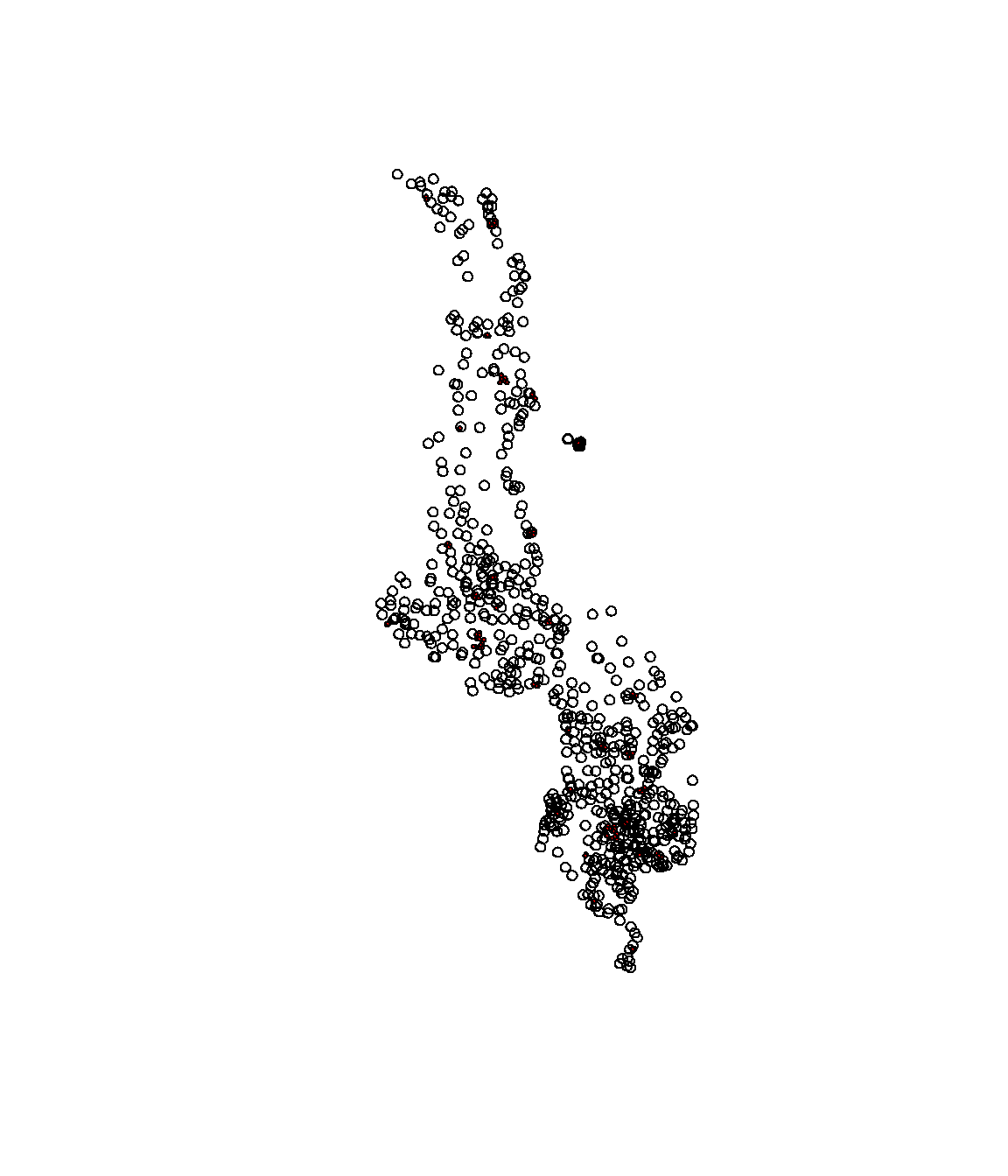
Hence, we decided to use the buffer areas instead of the point locations (GPS coordinates) to standardise/ minimise the measurement error from the off-setting of the coordinates, and in turn, use the buffer area to identify the probable EAs where the households may be located. Here we added a buffer around each of the GPS locations that account for the 2km and 5km displacement in urban and rural respectively. In that sense, we are assuming that each HHs can be in any place with that buffered area.

Code

#  Generating the offset buffer

for(i in 1:nrow(GPS)){

# Assigning buffer size (in m) acc. to Urban (U) or Rural (R)
offset.dist<-ifelse(GPS$URBAN_RURA[i]=="U", 2000, 5000)

# Generating the buffers around the centroids
GPS$buffer[i] <- st_buffer(GPS$geometry[i], dist = offset.dist)

}

Checking the results of the displacement buffers

Code

# Transforming the list into spatial class
GPS$buffer <- st_as_sfc(GPS$buffer)

# Checking that the output
plot(GPS$buffer) # Plotting the buffer
plot(GPS$buffer[GPS$URBAN_RURA == "U"],col='red',add=TRUE) # colouring red those that are urban (smaller radius)

Final cleaned dataset () and the spatial information (GPS) are merged andwas stored in: data/inter-output/dhs-gps.rds

Code

# Then the GPS w/ the geometry and buffer and the DHS data 
EligibleDHS <- left_join(EligibleDHS, GPS) 

# Saving DHS + GPS dataset into R object 
saveRDS(EligibleDHS, file=here::here("data", "inter-output","dhs_se_gps.rds"))

Then, the next step will be to combine with the information on maize Se at different aggregation level.

This will be done using the script 00_cleaning-locations.R.

2.5 Limitations

2.5.1 Limitations of DHS data

Time influence: DHS survey was performed in 2015 while GeoNut was in 2018 and Chilimba in 2009. However, we could assume that the Se concentration would have been remain fairly similar over time (REF, REF).
Seasonal variation: DHS survey was performed during Feb.- which are normally referred as the “hunger season” were food intake is at its lowest and food patterns and behaviours may be influenced by maize scarcity (at HH level). Including, other crop intakes and unrefined/ maize bran flour intake. However, according to previous studies, food patterns (related to maize intake) were fairly constant between IHS3-IHS5.

2.5.2 Limitation to DHS-MNS data

Cluster level data: Most our analysis are based on location, however, we only have location information at cluster level. This would mean that when comparing with the maize values, those values will be the same for all the women within one cluster. We may need to account for it in our model design: for instance by adding the cluster as random effect. Additionally, we need to check the variation within cluster as this will affect our model selection and results.
Displacement of the GPS coordinates at cluster level. This led to high chances of missclassification and reducing the accuracy of the results for small area (e.g., EAs). It also led to the reduction of the no. of co-located (maize Se & plasma Se) samples.
Confounding effect for certain variables: For instance, in the central and southern regions the women who were tested positive in malaria, where on average younger that those who were negative (see Section 2.1.3).